Conformers

The Amsterdam Modeling Suite contains a Conformers utility program that allows easy generation and manipulation of sets of molecular conformations:

• Generation of conformer sets from an initial geometry.

• Merging of conformer sets with a variety of equivalence comparison methods.

• Geometry optimizations of conformer sets with higher-level engines.

• Calculations of properties (e.g. spectra) for conformers from a set.

By coupling to the AMS driver, all of the above can be done using any engine available in AMS.

In this tutorial you will learn to:

• Generate a conformer set for 1,2-Propylene glycol (with the ForceField engine)

• Optimize and re-score the conformer set with a higher level of theory (with the DFTB and ADF engines)

• Calculate Boltzmann averaged properties such as IR, UV/Vis and NMR spectra.

See also

For a detailed description of the methods and options of the Conformers utility, see the Conformers page in the AMS driver manual.

Generate a conformer set

1. Start AMSinput

2. Obtain “1,2-Propylene glycol” using the button or by copy-pasting its SMILES string into AMSinput: CC(O)CO

Once we have our molecule, we just need to set up the options for the Conformers tool:

1. In AMSinput, select the Conformers panel: → .

2. Make sure that Task is set to Generate.

3. In the Filter section, tick the box next to Remove non minima.

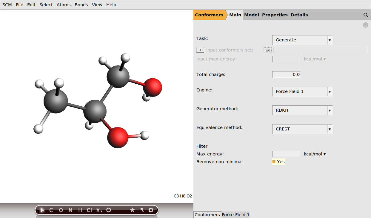
Note that we are using the RDKit generator here, which uses the RDKit library to generate a set of randomized molecular geometries. These are then optimized using the AMS driver and the chosen engine (in this case, the default ForceField engine is used) and duplicates discarded to yield a set of unique conformers. Finally, thanks to us ticking the Remove non minima box, a PES point characterization is performed on each structure to ensure that it is indeed a minimum on the potential energy surface. Otherwise it could happen that the optimization accidentally converges to a transition state, which would then be included in our conformer set. It is generally good practice to enable this option when using fast engines, where the computational cost of the PES point characterization is not a problem.

This concludes the setup of the job. We can now save and run it!

1. Click File → Run in the menu bar.

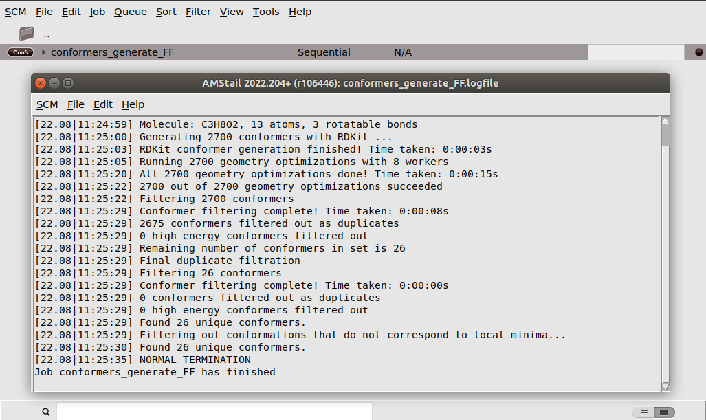
2. When asked to save the job, call it conformers_generate_FF.

3. AMSjobs will come to the front. Click the two lines below your job to open its logfile in AMStail.

If you watch the logfile while the job is running, you will see that the initial randomization of the geometries with RDKit is very quick, and that most time is spent in the geometry optimizations. However, the job should be pretty quick to run.

Once the job has finished, AMSinput will come to the front and ask you if you want to use the conformers.rkf file of the finished calculation to set up another calculation. You can choose Yes here, as this is exactly what we will do in the next part of the tutorial. However, let us first have a look at the conformers we found. The obtained conformer set can be visualized and inspected in AMSmovie.

With the job selected in AMSjobs, click SCM → Movie in the menu bar.

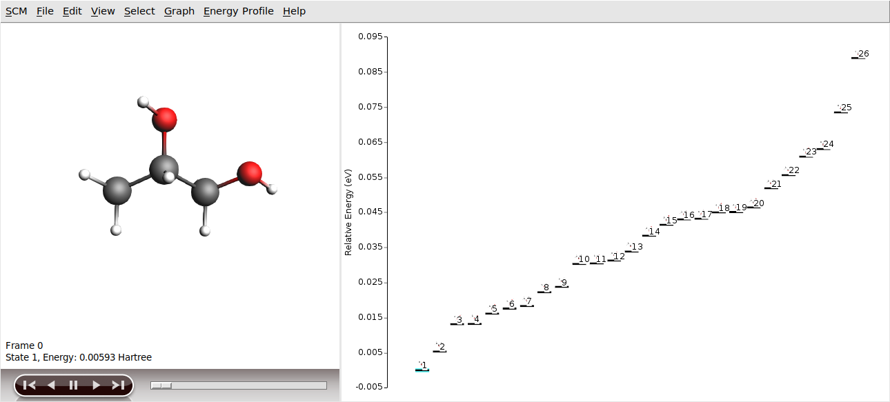
There are 26 conformers to be found with the ForceField engine for 1,2-Propylene glycol.

Get a better view of the lowest energy conformers: on the right-hand side, zoom in to the area of interest. You can go through the conformers using the arrow keys or by clicking on the horizontal bars

Getting more accurate conformers geometries and energies

The conformers we just generated were optimized using the (default) ForceField engine. While the Force Field engine is computationally very fast, the conformers geometries and energies will not be very accurate.

For practical applications, you may need more accurate geometries and energies. This can be achieved in two ways:

Directly generate with an accurate engine

You can directly generate the conformers using a more accurate engine, e.g. the DFT engine ADF. In the Conformers panel, set Task to Generate. Select an accurate engine (e.g. Engine → ADF) and then configure the details of the engine by clicking on the tab at the bottom of the panel (e.g. ADF 1). This is easy to set up, but can be computationally very expensive to run, since the conformer tool will run thousands of Geometry Optimization under the hood.

Generate with fast engine and refine with accurate engine

An alternative, computationally cost-effective approach is to take the conformers generated with a lower level of theory engine and refined them with a more accurate engine.

In the next section we will illustrate this second method by taking the conformers we just generated using the ForceField engine and then:

• optimize the conformers generated with the ForceField engine using the more accurate DFTB engine

• score the conformers optimized with DFTB engine using energies from the more accurate ADF engine

Optimization and scoring at higher level of theory

Next step is to improve the geometries and energies of the conformers we have found.

The Optimize task of the conformer tool is intended for this: it will perform a geometry optimization on each of the conformers in the set and will filter out duplicates in the end. (You may get duplicates at this point if multiple conformers from the original set collapse into the same minimum at the new level of theory.)

1. Switch back to AMSinput and the main panel.

2. Set Task → Optimize.

3. Click on the folder button next to Input conformer set and select the main output file from the previous job: conformers_generate_FF.results/conformers.rkf (If you clicked Yes in the popup window earlier, this will already be filled in.)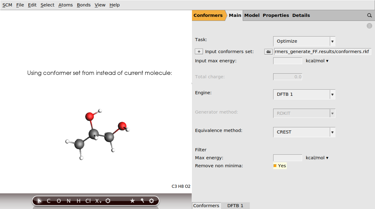

4. Set Engine → DFTB.

In this tutorial we will use default settings for the DFTB engine, but in general you may want to adjust the engine’s settings. To navigate to the Engine’s panel, click the DFTB 1 tab at the bottom of the panel. To go back to the Conformers main panel, click on Conformers at the bottom of the panel.

We can now save and run the calculation:

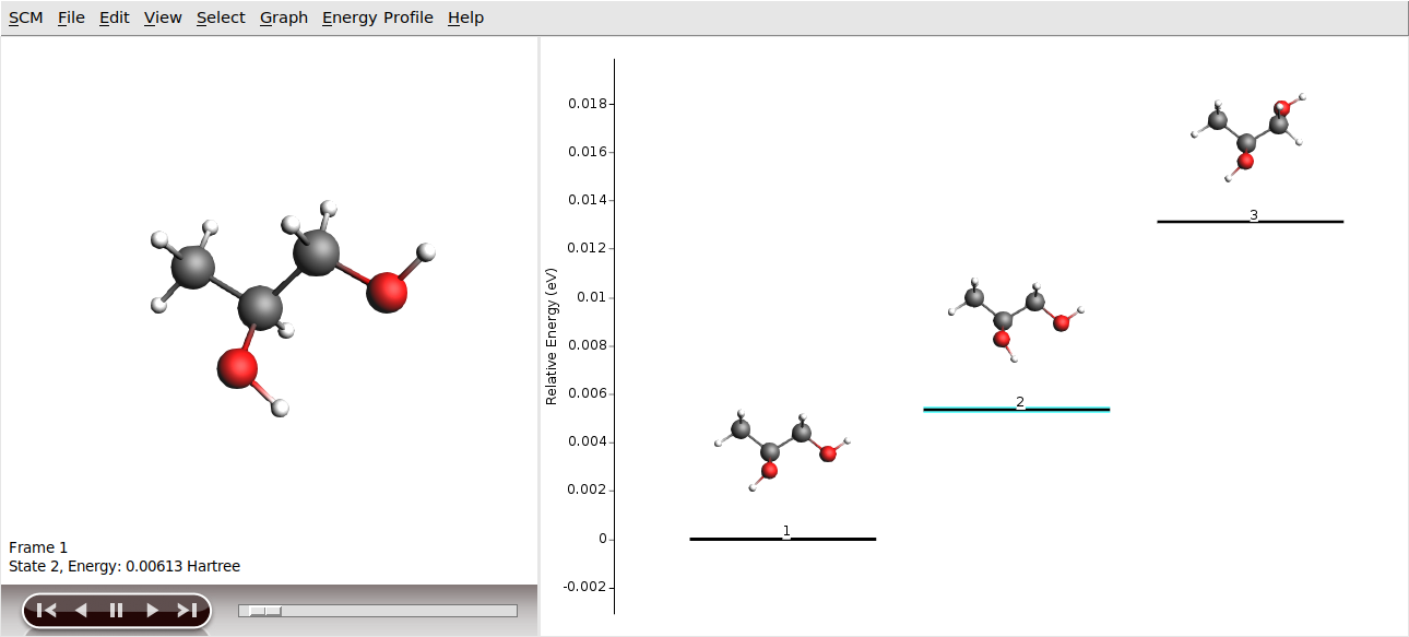
1. Click File → Save As… in the menu bar and save the job as conformers_optimize_DFTB.

2. Click File → Run.

3. When asked to use the conformers.rkf file in AMSinput, click Yes.

Wait for the job to finish (it should rather quick) and open the results in AMSMovie:

With the conformers_optimize_DFTB job selected, click SCM → Movie in the menu bar.

You may notice that after the DFTB optimization you end up with with fewer conformers than you started with. This is because some conformers that are distinct at the force-field level converge to the same local minimum when optimized using the DFTB engine (and are therefore removed as duplicate conformers).

It is important to keep in mind that different levels of theory might have different conformer sets: a conformation that is a local minimum at the force field level might not have an equivalent local minimum at the DFT level or vice-versa. It is therefore possible that you will miss out some of the conformers by following the multi-step-procedure outlined in this section. On the upside, this multi-step procedure is more than 1000 times faster than simply generating conformers using the ADF engine.

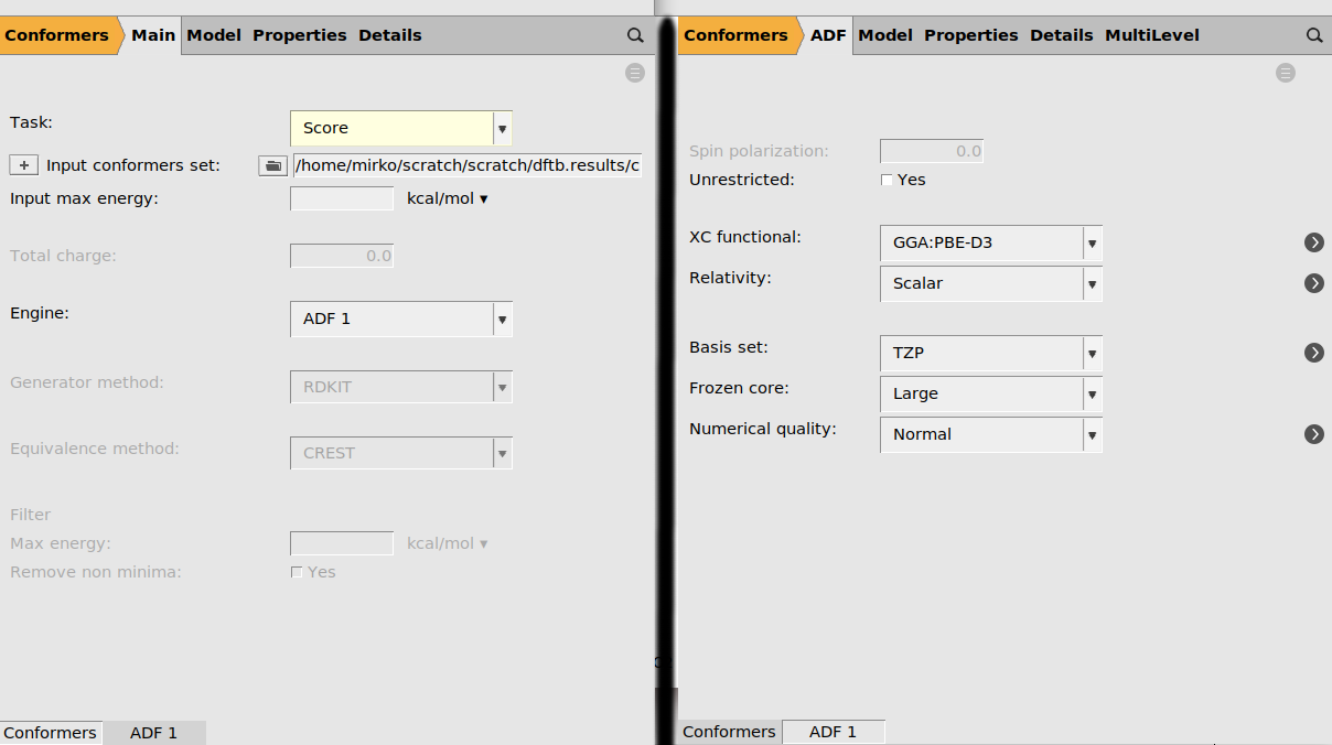
Finally, we can use the Score task to perform a single point calculation at the DFT level on the DFTB-optimized conformer set:

1. Switch back to AMSinput and the main panel.

2. Set Task → Score.

3. Make sure the Input conformer set is set to the main output file from the previous job: conformers_optimize_DFTB.results/conformers.rkf. (If this is not the case click the folder button next to Input conformer set and select it in the dialog.)

4. Set Engine → ADF

Let us now configure the details of the used engine:

1. Click the ADF 1 tab at the bottom of the panel

2. Select XC functional → GGA-D → PBE-D3

3. Select Basis set → TZP

1. Click File → Save As… in the menu bar and save the job as conformers_scored_ADF.

2. Click File → Run.

3. When asked to use the conformers.rkf file in AMSinput, click No. (We will proceed with the DFTB results in the next step of this tutorial.)

When the calculation is finished, open and visualize the results with AMSMovie:

With the conformers_scored_ADF job selected, click SCM → Movie in the menu bar.

Boltzmann weighted IR spectra

Starting from a previously generated conformers set, you will now learn how to calculate Boltzmann weighted IR spectra. For the purpose of this tutorial we will use the DFTB optimized set of conformers and calculate the spectrum at the DFTB level.

1. Open a new AMSinput window by clicking SCM → New Input in the menu bar.

2. Select the DFTB panel: → .

3. Click Model → Coordinates in the right menu bar.

4. Select Use → Selected File.

5. Click the folder button next to Molecule from: and select the conformer set we obtained from the DFTB optimization step earlier: conformers_optimize_DFTB.results/conformers.rkf

6. Click on the next to Use → Selected File to go to the corresponding details panel.

7. Select Use systems from → Conformers.

Whatever job we now set up will be repeated for each conformer from the selected set. As all the structures in the set have already been optimized, we just need to run a single-point calculation on each conformer now, for which we enable the calculation of all the desired spectra.

1. Switch back to the main DFTB panel by clicking Main in the right menu bar.

2. Select Task → Single Point.

3. Tick the Frequencies check-box.

Note

Technically you could select Task → Geometry Optimization and then first optimize the geometries of the set before calculating the spectra. However, no filtering for duplicates takes place after the optimizations, so if two conformers would then collapse to the same minimum we would double count them in the calculation of the spectra. We therefore recommend to always optimize conformer sets with the Optimize task of the Conformers tool.

We are now ready to run these jobs!

1. Click File → Save As… in the menu bar and save the job as conformers_spectra_DFTB.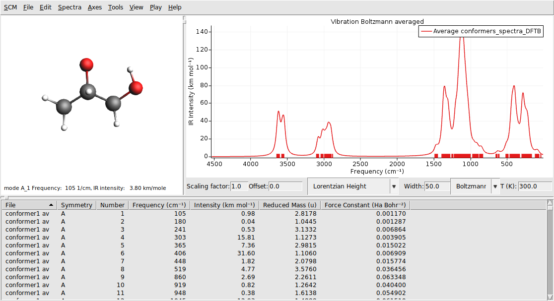

2. Click File → Run.

3. Click No in the AMSinput pop-up window.

4. Open the IR spectrum by clicking SCM → Spectra.

The IR spectra of the different conformers contribute to the total spectrum according to their Boltzmann weights. You can change the temperature that is used for the Boltzmann distribution in the field on the right. Let us add the IR spectrum of the pure lowest energy conformer to our graph, to see how the Boltzmann averaged spectrum differs from the spectrum of a single conformer.

Click File → Add and select the conformer1/dftb.rkf file.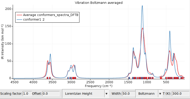

Try setting the Boltzmann temperature to 0K: as expected the two spectra will then overlap, as only the lowest energy conformer contributes at 0K. Feel free to add the individual spectra of other conformers to get an idea on how much the IR spectrum depends on the conformation.

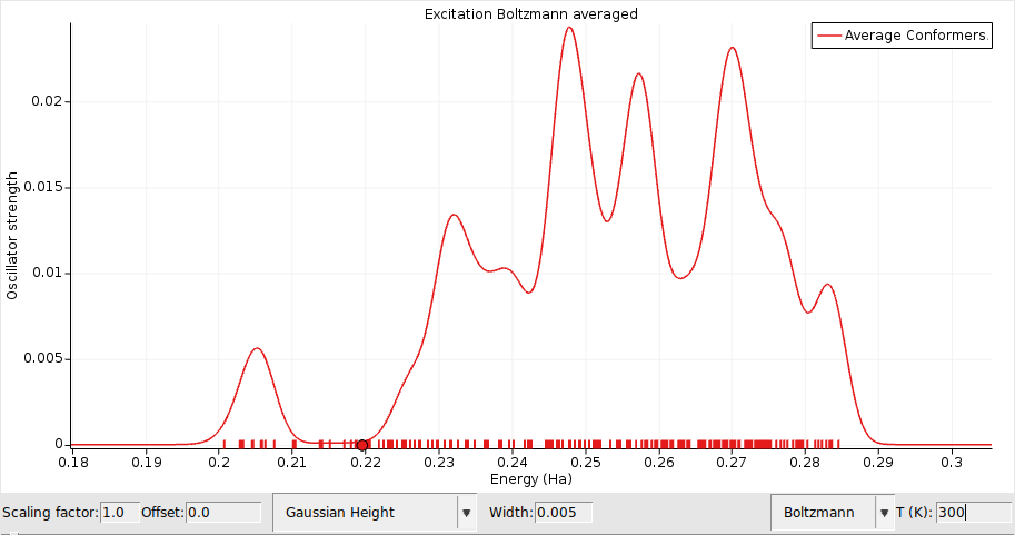
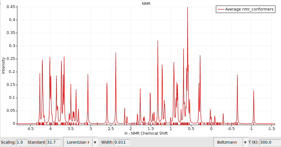
Boltzmann weighted H-NMR or UV/Vis spectra

Similarly we can compute Boltzmann weighted NMR or UV/Vis spectra using the ADF engine.

Let’s first set up the calculation details for the ADF engine depending on which property you want to calculate:

UV/VisH-NMR

1. Open a new AMSinput window by clicking SCM → New Input in the menu bar.

2. In the main ADF panel select XC functional → GGA → PBE and Basis set → TZP

3. Go to the panel Properties → Excitations (UV/Vis), CD

4. Select Type of excitations: → AllowedOnly

Now we select the conformer set we computed earlier on:

1. Click Model → Coordinates in the right menu bar.

2. Select Use → Selected File.

3. Click the folder button next to Molecule from: and select the conformer set we obtained from the DFTB optimization step earlier: conformers_optimize_DFTB.results/conformers.rkf

4. Click on the next to Use → Selected File to go to the corresponding details panel.

5. Select Use systems from → Conformers.

Save and run:

1. Click File → Save As… in the menu bar and give the job an appropriate name.

2. Click File → Run.

3. Wait for the calculation to finish (this might take a few minutes) and visualize the spectrum by clicking on SCM → Spectra.

UV/VisH-NMR