Using AMS as an ASE Calculator
This example illustrates how to use the AMS ASE calculator with ASE’s BFGS geometry optimizer driven by AMS-calculated forces.
Use this workflow only when you specifically need ASE. If you just want to run a normal AMS single-point or geometry optimization from Python, it is simpler to use PLAMS directly, as in Getting Started: Geometry Optimization of Water.
In this example, the AMS driver is effectively replaced by ASE tools while AMS engines such as ADF, BAND, DFTB, or ForceField still provide the energies and forces.
Initial imports
from scm.plams import *
from scm.plams.interfaces.adfsuite.ase_calculator import AMSCalculator
from ase.optimize import BFGS
from ase.build import molecule as ase_build_molecule
import matplotlib.pyplot as plt

# In this example AMS runs in AMSWorker mode, so we have no use for the PLAMS working directory
# Let's delete it after the calculations are done
config.erase_workdir = True
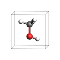
Construct an initial system
Here, we use the molecule() from ase.build to construct an ASE Atoms object.
You could also convert a PLAMS Molecule to the ASE format using toASE().
atoms = ase_build_molecule("CH3OH")
# alternatively:
# atoms = toASE(from_smiles('CO'))

atoms.set_pbc((True, True, True))  # 3D periodic
atoms.set_cell([4.0, 4.0, 4.0])  # cubic box

view(fromASE(atoms), height=200, width=200, guess_bonds=True, direction="tilt_z")
Set the AMS settings
First, set the AMS settings as you normally would do:
s = Settings()
s.input.ams.Task = "SinglePoint"  # the geometry optimization is handled by ASE
s.input.ams.Properties.Gradients = "Yes"  # ensures the forces are returned
s.input.ams.Properties.StressTensor = "Yes"  # ensures the stress tensor is returned

# Engine definition, could also be used to set up ADF, ReaxFF, ...
s.input.ForceField.Type = "UFF"

# run in serial
s.runscript.nproc = 1
Run the ASE optimizer
print("Initial coordinates:")
print(atoms.get_positions())

with AMSCalculator(settings=s, amsworker=True) as calc:
    atoms.calc = calc
    optimizer = BFGS(atoms)
    optimizer.run(fmax=0.27)  # optimize until forces are smaller than 0.27 eV/ang

print(f"Optimized energy (eV): {atoms.get_potential_energy()}")
print("Optimized coordinates:")
print(atoms.get_positions())
Initial coordinates:
[[-0.047131  0.664389  0.      ]
 [-0.047131 -0.758551  0.      ]
 [-1.092995  0.969785  0.      ]
 [ 0.878534 -1.048458  0.      ]
 [ 0.437145  1.080376  0.891772]
 [ 0.437145  1.080376 -0.891772]]
      Step     Time          Energy         fmax
BFGS:    0 10:46:19        0.424475        3.0437
BFGS:    1 10:46:19        0.354817        2.8239
... output trimmed ....
BFGS:    4 10:46:19        0.200223        0.5503
BFGS:    5 10:46:19        0.196200        0.1861
Optimized energy (eV): 0.19620006656661387
Optimized coordinates:
[[-7.36222829e-02  6.46660224e-01  1.80595127e-17]
 [-4.27710560e-02 -7.22615924e-01 -7.74061622e-18]
 [-1.12651815e+00  9.85598502e-01 -2.86803391e-18]
 [ 9.22587449e-01 -9.45309675e-01 -3.18423479e-18]
 [ 4.42945518e-01  1.01179194e+00  9.09790370e-01]
 [ 4.42945518e-01  1.01179194e+00 -9.09790370e-01]]
See also
Python Script
#!/usr/bin/env python
# coding: utf-8

# ## Initial imports

from scm.plams import *
from scm.plams.interfaces.adfsuite.ase_calculator import AMSCalculator
from ase.optimize import BFGS
from ase.build import molecule as ase_build_molecule
import matplotlib.pyplot as plt

# In this example AMS runs in AMSWorker mode, so we have no use for the PLAMS working directory
# Let's delete it after the calculations are done
config.erase_workdir = True


# ## Construct an initial system
# Here, we use the ``molecule()`` from ``ase.build`` to construct an ASE Atoms object.
#
# You could also convert a PLAMS Molecule to the ASE format using ``toASE()``.

atoms = ase_build_molecule("CH3OH")
# alternatively:
# atoms = toASE(from_smiles('CO'))

atoms.set_pbc((True, True, True))  # 3D periodic
atoms.set_cell([4.0, 4.0, 4.0])  # cubic box

view(fromASE(atoms), height=200, width=200, guess_bonds=True, direction="tilt_z", picture_path="picture1.png")


# ## Set the AMS settings
#
# First, set the AMS settings as you normally would do:

s = Settings()
s.input.ams.Task = "SinglePoint"  # the geometry optimization is handled by ASE
s.input.ams.Properties.Gradients = "Yes"  # ensures the forces are returned
s.input.ams.Properties.StressTensor = "Yes"  # ensures the stress tensor is returned

# Engine definition, could also be used to set up ADF, ReaxFF, ...
s.input.ForceField.Type = "UFF"

# run in serial
s.runscript.nproc = 1


# ## Run the ASE optimizer

print("Initial coordinates:")
print(atoms.get_positions())

with AMSCalculator(settings=s, amsworker=True) as calc:
    atoms.calc = calc
    optimizer = BFGS(atoms)
    optimizer.run(fmax=0.27)  # optimize until forces are smaller than 0.27 eV/ang

print(f"Optimized energy (eV): {atoms.get_potential_energy()}")
print("Optimized coordinates:")
print(atoms.get_positions())