4.2. Train MACE with the ParAMS GUI

Important

This tutorial is only compatible with ParAMS 2027.1 or later.

This example shows how to train your own MACE machine learning potential by fine-tuning/retraining the MACE-MP-0-Small foundation model. The settings in this tutorial follow the recommendations in:

Tamás Lajos Tompa, Eszter Varga-Umbrich, Ilyes Batatia, Alin M. Elena, Noam Bernstein and Gábor Csányi, Fine-tuning MLIP foundation models: strategies for accuracy and transferability, arXiv:2606.12704 (2026), https://doi.org/10.48550/arXiv.2606.12704.

See also

Train M3GNet with the ParAMS GUI

Train an M3GNet Potential with ParAMS

Prerequisite: Follow the Getting Started: Lennard-Jones and Import training data (GUI) tutorials to get familiar with the ParAMS GUI.

In this tutorial, the training data has already been prepared.

In general, when training ML potentials like MACE you can only train to single-point energy and forces. For details, see Requirements for job collection and data sets.

4.2.1. Open the example input file

Open the ParAMS GUI: SCM → ParAMS

Click on the yellow Optimization panel on the left hand side. This expands the panel.

Click on the yellow Optimization again, and choose Machine Learning in the drop-down menu

Click on Backend in the panel, and choose MACE in the drop-down menu

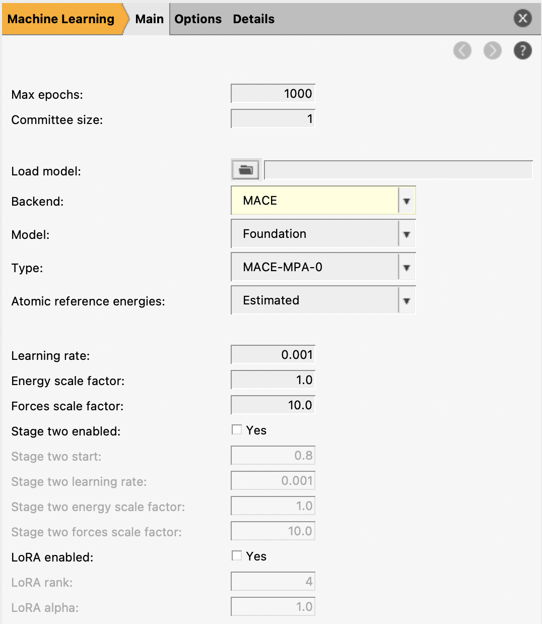
You should now see input options for MACE in the Machine Learning.

Open the example input file: File → Open and browse to params.in

You can also find this file in $AMSHOME/scripting/scm/params/examples/MACE/params.in.

This loads a few different composition of oxygen doped lithium argyrodite (LPSC) and sets up some ML training settings.

Important

The set of elements supported by a MACE model is determined by the training data. Any elements not present in the training set are removed from the model and cannot be used later.

In this tutorial, since the training data contains only lithuim, sulfur, chlorine, phosphorous and oxygen, the retrained potential will only be valid for systems containing these atoms. To build a model that supports multiple elements, make sure all required elements are present in the training data.

4.2.2. Job collection, training and validation sets

For training machine learning potentials, you can only train to single-point energy and forces.

Switch to the Jobs panel

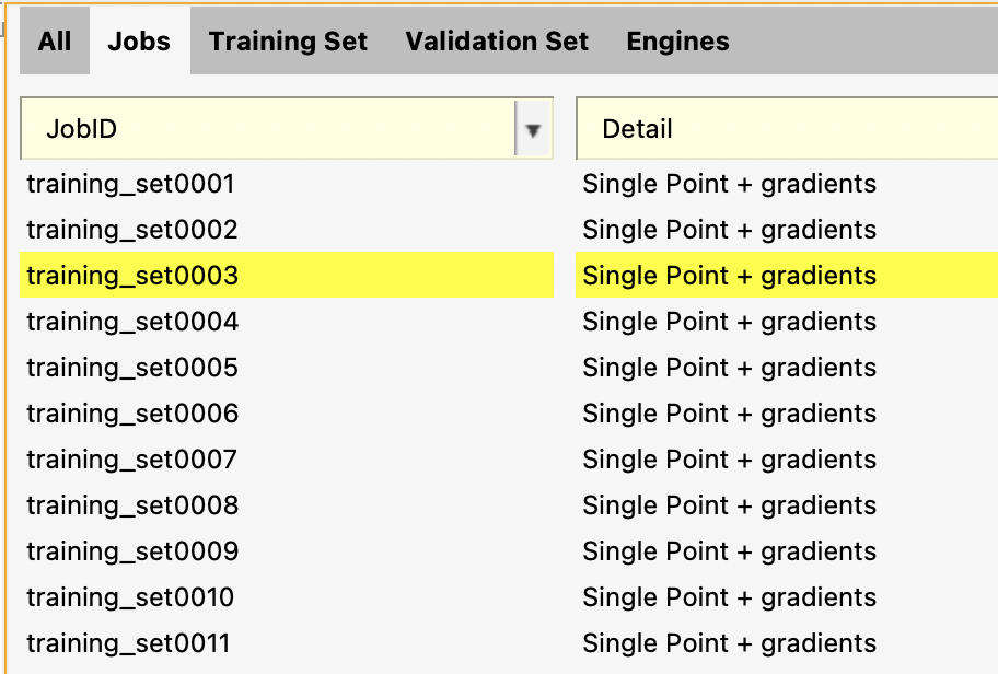
Here, you see that all jobs are of type “Single Point + gradients”. This is the only type of job that can be used during the training. The job collection can also contain other types of jobs, but they will then not be used during the training but will simply be run after the training has finished.

Tip

When importing training data into ParAMS:

• Use the “add trajectory singlepoints” importer to import data from trajectories

• Use the “add pesscan singlepoints” importer to import data from PES scans

• If you use the “add single job” importer, make sure that “Task (for new job)” is set to singlepoint !

Switch to the Training set panel

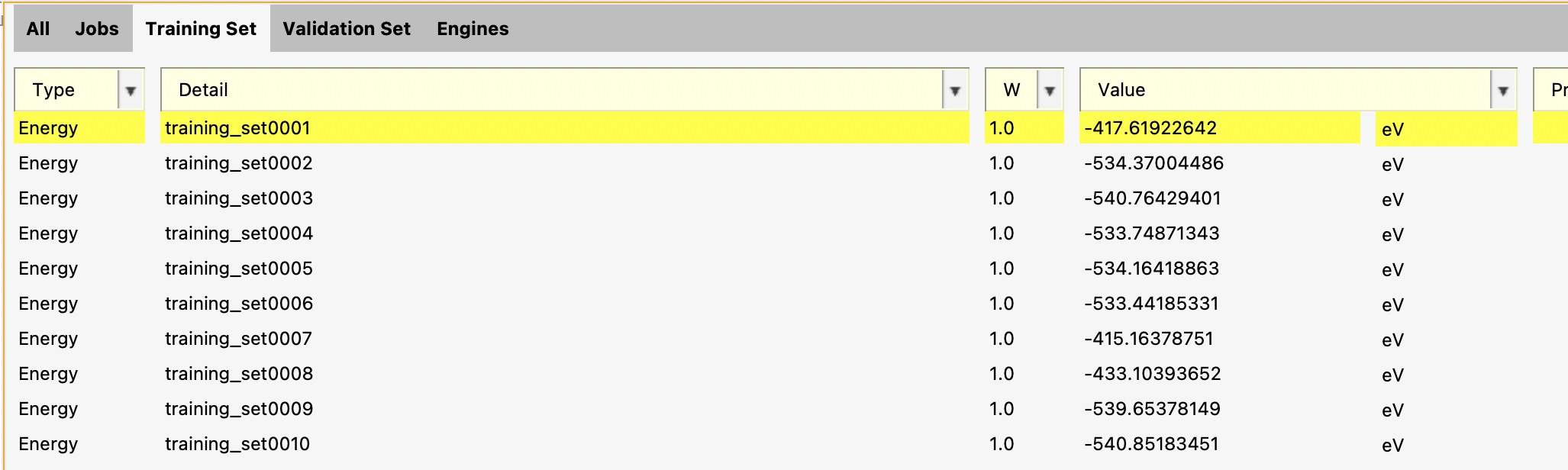
Here, you can see energies and forces for the training set.

Switch to the Validation set panel

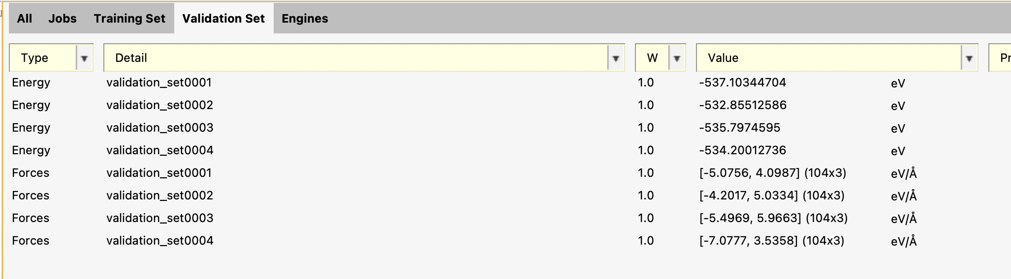
Here, you can see energies and forces for the validation set.

For task Machine Learning, you should always have at least one entry in the validation set.

Note

The energy and forces for a given job must belong to the same data set.

Example: Both the energy and forces for validation_set0001 are in the validation set. It is not allowed to split these so that for example the energy is in the training set and the forces in the validation set.

4.2.3. Machine learning settings

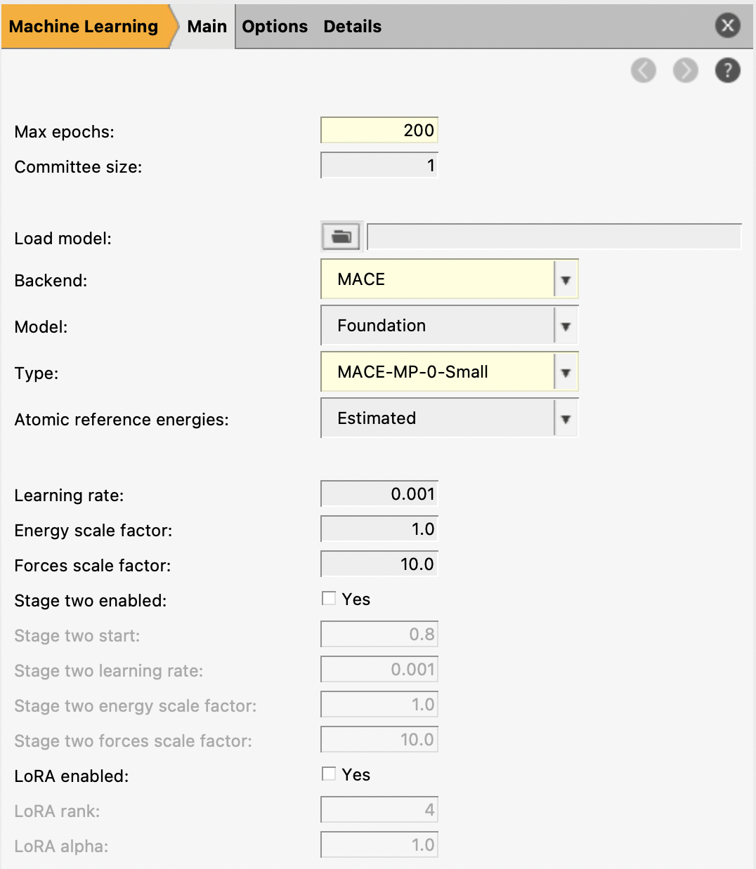
The bottom left panel shows the machine learning settings.

• Max epochs: sets the maximum number of training epochs (full passes over the training dataset). In practice, the optimal number may be lower if early stopping is triggered or the validation error plateaus. Increasing this allows the model more opportunity to converge, but excessively large values can lead to overfitting or unnecessary computational cost.

• Committee size: specifies how many independent ML models are trained with different initializations. The final prediction is obtained by averaging over all models in the committee. Using a committee (size > 1) can improve robustness and provides a useful estimate of prediction uncertainty (via the spread between models), but increases both computational time and memory usage roughly linearly with the number of models.

• Load model: allows you to initialize training from an existing model stored in a ParAMS results directory. This enables continuing training (e.g., for more epochs), fine-tuning on additional data, or adapting a model to a new system. This is particularly useful for transfer learning workflows, such as refining a pretrained model on a specific dataset.

• Backend: selects the machine learning model architecture used for training. Here we use MACE, a message-passing neural network designed for atomistic systems. Note that MACE must be installed separately via the AMS package manager (SCM → Packages) before it can be used.

• Atomic reference energies: sets the isolated-atom reference energies (E0s) used by MACE. Use Estimated when fine-tuning a foundation model unless you have computed explicit isolated-atom energies at the same level of theory as the training data.

• Learning rate: controls the step size used during optimization. Larger values allow faster learning but may lead to instability or overshooting, while smaller values provide more stable and precise convergence but can slow down training.

• Stage two: optionally changes the MACE loss weights and learning rate partway through training. This can be useful when training a custom MACE model from scratch, where the first stage can emphasize forces and the second stage can refine the energy scale. For fine-tuning a foundation model, leave two-stage training disabled unless validation results show a clear need to change the energy/forces balance.

• LoRA: enables Low-Rank Adaptation, a parameter-efficient fine-tuning technique that freezes the pretrained model’s weights and instead trains only small low-rank correction matrices injected into each layer, controlled by the Rank (the size of the correction) and Alpha (its scaling). Try regular fine-tuning first. LoRA can help reduce overfitting and catastrophic forgetting when fine-tuning on small datasets, but it can limit accuracy when the target system differs strongly from the pretrained model.

For the MACE backend, you can select three different Models:

• Custom: this trains a new neural network completely from scratch. You can decide the architecture for this neural network, for example the distance cutoff and the number of channels. Note that you will typically require quite a lot of training data to train a good model using Custom.

• Foundation: this starts the training from one of the pretrained MACE models. This typically makes training much faster. You cannot, however, change the architecture parameters.

• Model File: this starts the training from a custom pretrained MACE model (for example, a previous retraining or MACE model not available in AMS).

When training a Custom MACE model from scratch, other optimizer hyperparameters may also need to be changed from the fine-tuning-oriented defaults. Common from-scratch starting points are a learning rate of 1e-2, EMA decay of 0.99, and gradient clipping of 10.0. Here you will fine-tune a foundation model.

Set Max epochs to 200.

Set Model to Foundation.

Set Type to MACE-MP-0-Small.

Keep Atomic reference energies set to Estimated and leave Stage two enabled and LoRA enabled unchecked.

In the bottom left panel, switch to Options → Loss Function

Here the forces and energy coefficients can be set for the loss function.

In addition, in the main machine learning panel, you can set the Energy scale factor and the Forces scale factor. These are applied to the above energy and forces coefficients, such that the final coefficients are the product of these two settings.

For this tutorial, leave the default scale factors unchanged. With the default loss coefficients, this gives an overall energy loss weight of 10 and an overall forces loss weight of 10.

4.2.4. Run the MACE training

File → Save As, and save the job with the name mace_tutorial.params

File → Run (or run the job from AMSjobs)

Wait for the job to finish. It may take a few minutes.

4.2.5. View the MACE training results

In the bottom right panel, select the Graphs tab

Change the right-most graph by clicking the drop-downs and selecting e.g. Stats: Energy and MAE

Here, you can see graphs for loss function and stats vs. epoch.

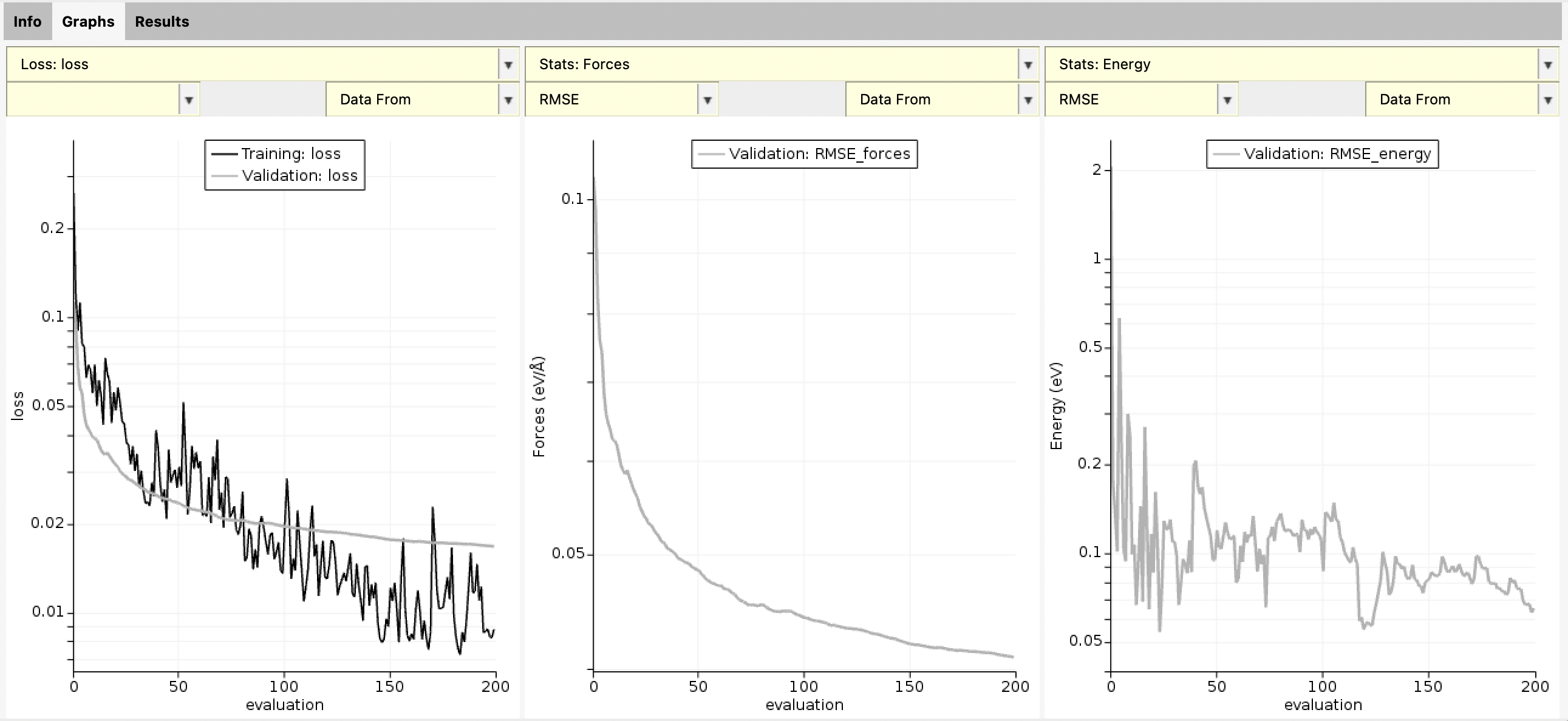
The training and validation curves should decrease and then level off. If the validation error starts to increase while the training error keeps decreasing, the model may be overfitting.

At the end of the training, you also get a scatter plot with predicted vs. reference forces and energies. You can switch between Best training and Best validation to see the training and validation performance.

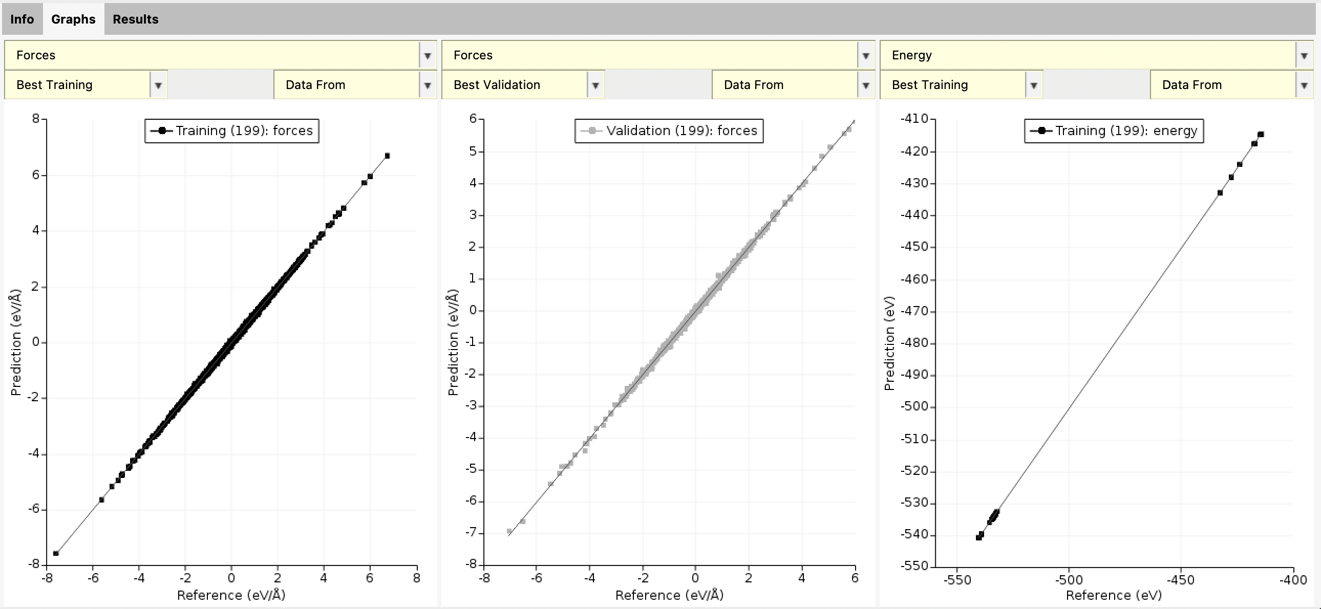
For this small model and dataset, you can see that the agreement is good.

Note

For Task MachineLearning, the scatter plot only appears when the training has finished.

4.2.6. Use the retrained model for production calculations

In the bottom right panel, select the Results tab

In the drop-down, select Validation best: engine (or Training best: engine)

This shows the contents of part of the AMS text input file you would need to provide to use the retrained model in a production calculation. In particular, it shows you the ParameterFile containing the trained parameters.

There are two ways to import these engine settings into AMSinput:

4.2.6.1. Method 1: Open optimized engine in AMSinput

File → Open Optimized Engine in AMSinput → Best Validation

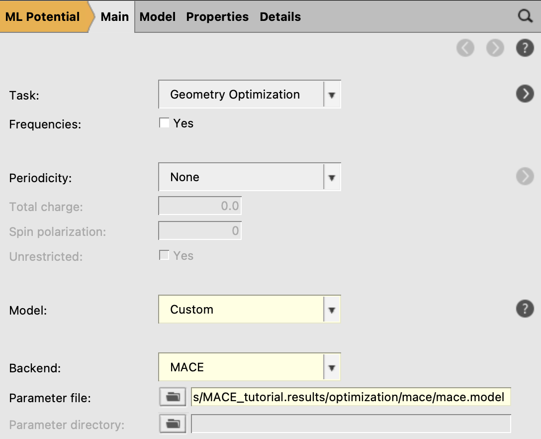
This opens a new AMSinput window with the MLpotential engine selected. This gives you a warning to double-check the input. It should switch automatically to the MLpotential engine with Model Custom and set the corresponding ParameterFile.

4.2.6.2. Method 2: Copy-paste into AMSinput

Select the entire Engine MLPotential … EndEngine block

Edit → Copy

SCM → New Input

In the newly opened AMSinput window: Edit → Paste

This gives you a warning to double-check the input. It should switch automatically to the MLpotential engine with Model Custom and set the corresponding ParameterFile.

4.2.7. Optional next steps

4.2.7.1. Try LoRA fine-tuning

LoRA can be useful when you have a small fine-tuning data set and want to train fewer parameters. It keeps most pretrained weights fixed and trains small low-rank adapters instead. This can reduce overfitting, but it can also limit the final accuracy if the target system differs strongly from the foundation model.

To try LoRA, set LoRA enabled to Yes. The default LoRA rank of 4 and LoRA alpha of 1 are a reasonable starting point. Compare the validation errors and test behavior against regular fine-tuning before using the model for production calculations.