Linear Transit, PES scan¶

Optimizing PES scan¶

In optimizing mode, each PES point is treated as a constrained optimization:

• AMS creates constraint descriptors for the scanned coordinate value(s) at that point.

• The geometry optimizer relaxes all other degrees of freedom subject to these constraints.

• If you specify additional constraints in the global Constraints block, those are included too.

• The optimizer is configured via the GeometryOptimization block.

Non-optimizing (rigid) PES scan¶

In non-optimizing mode, AMS does not run the optimizer at all.

• For each PES point, AMS starts from the geometry of the previous point (or the initial geometry for the first point).

• It then directly sets the requested scan coordinate value(s) (distance/angle/dihedral/coordinate) by manipulating the geometry in internal-coordinate space.

• Finally, AMS runs a single point calculation for that geometry.

Distance, angle, and dihedral angle coordinates¶

The coordinate descriptors are very similar to the constraint descriptors in the Constraints block used by the geometry optimization task, but are followed by two values delimiting the start and end of the coordinates, instead of just a single value:

Coordinate atomIdx [x|y|z] startValue endValue

Moves the atom with index atomIdx (following the order in the System block) along a Cartesian coordinate (x, y or z), starting at startValue and ending at endValue (given in Angstrom).

Note

In non-optimizing mode (Optimize False), this coordinate is applied as a rigid translation of the entire molecule/fragment containing that atom along the requested Cartesian direction, rather than moving a single atom through the structure.

Distance atomIdx1 atomIdx2 startDist endDist

Scans the distance between the atoms with index atomIdx1 and atomIdx2, starting from startDist and ending at endDist, both given in Angstrom.

Note

In non-optimizing mode, AMS determines the moving atoms from the bond network (conceptually: one side of the bond graph moves relative to the other). This works best when the A-B connection separates the system into two parts.

Angle atomIdx1 atomIdx2 atomIdx3 startAngle endAngle

Scans the angle (1)–(2)–(3) between the atoms with indices atomIdx1-3, as given by their order in the System%Atoms block. The scanned angle starts at startAngle and ends at endAngle, given in degrees.

Dihedral atomIdx1 atomIdx2 atomIdx3 atomIdx4 startAngle endAngle

Scans the dihedral angle (1)–(2)–(3)–(4) between the atoms with indices atomIdx1-4, as given by their order in the System%Atoms block. The scanned dihedral starts at startAngle and ends at endAngle, given in degrees.

SumDist atomIdx1 atomIdx2 atomIdx3 atomIdx4 start end

Scans the sum of the distances R(1,2)+R(3,4) between the atoms with indices atomIdx1-4, as given by their order in the System%Atoms block. The values to be scanned start at start and end at end, given in Angstrom.

DifDist atomIdx1 atomIdx2 atomIdx3 atomIdx4 start end

Scans the difference between the distances R(1,2)-R(3,4) of the atoms with indices atomIdx1-4, as given by their order in the System%Atoms block. The values to be scanned start at start and end at end, given in Angstrom.

Joint scan coordinates¶

Note that multiple of these coordinate descriptors can be combined within a single ScanCoordinate block. This combines the individual coordinates into one compound coordinate, i.e. all coordinates will transit together through their respective ranges. In this way the symmetric stretch in water could be scanned by specifying the following single ScanCoordinate block (assuming that the oxygen atom is the first in the System%Atoms block):

ScanCoordinate
   Distance  1 2  0.8 1.1
   Distance  1 3  0.8 1.1
End

Multidimensional PES scan¶

A multidimensional PES scan can be performed by specifying multiple ScanCoordinate blocks in the input. To scan the space spanned by the bending and symmetric stretch modes in water, one would use the following scan coordinates:

ScanCoordinate
   Distance  1 2  0.8 1.1
   Distance  1 3  0.8 1.1
End
ScanCoordinate
   Angle  2 1 3  90 130
End

In principle an arbitrary number of ScanCoordinate blocks can be combined to specify the scanned configuration space. However, the total number of sample points is the product of the number of points along all coordinates, and hence grows quickly with the number of dimensions. Furthermore, only 1D (linear transit) and 2D PES scans can be visualized in the GUI. We therefore suggest sticking with <=2 dimensional PES scans.

Isotropic scaling of the unit cell volume or area¶

CellVolumeScalingRange startValue endValue

Isotropic scaling of the unit cell. Example: CellVolumeScalingRange 0.9 1.1 will scale the volume between 90% and 110% of the original unit cell. For 2D-periodic crystals, the area will be scaled instead.

CellVolumeRange startValue endValue

Isotropic scaling of the unit cell. Example: CellVolumeRange 300 500 will scale the volume between 300 ų and 500 ų for a 3d-periodic system. For 2D-periodic systems, the area will be scaled between 300 Ų and 500 Ų.

Scaling of the lattice vector lengths¶

These options keep the angles between lattice vectors fixed.

LatticeARange startValue endValue

Scans the length of the first lattice vector. Can be combined with the LatticeBRange and LatticeCRange keywords, but no other coordinates within the same ScanCoordinate. Unit: angstrom.

LatticeBRange startValue endValue

Scans the length of the second lattice vector. Can be combined with the LatticeARange and LatticeCRange keywords, but no other coordinates within the same ScanCoordinate. Unit: angstrom.

LatticeCRange startValue endValue

Scans the length of the third lattice vector. Can be combined with the LatticeARange and LatticeBRange keywords, but no other coordinates within the same ScanCoordinate. Unit: angstrom.

Strain matrix in Voigt notation¶

3D crystal: FromStrainVoigt xx yy zz yz xz xy, ToStrainVoigt xx yy zz yz xz xy

The FromStrainVoigt and ToStrainVoigt keywords need to be applied together. Example: FromStrainVoigt -0.1 -0.1 -0.1 -0.1 -0.1 -0.1 , ToStrainVoigt 0.1 0.1 0.1 0.1 0.1 0.1

2D crystal: FromStrainVoigt xx yy xy, ToStrainVoigt xx yy xy

The FromStrainVoigt and ToStrainVoigt keywords need to be applied together. Example: FromStrainVoigt -0.1 -0.1 -0.1 , ToStrainVoigt 0.1 0.1 0.1

1D crystal: FromStrainVoigt xx, ToStrainVoigt xx

The FromStrainVoigt and ToStrainVoigt keywords need to be applied together. Example: FromStrainVoigt -0.1 , ToStrainVoigt 0.1

Scan arbitrary lattices¶

Scan arbitrary lattices specifying the initial and final lattice vectors, using the same format as in the System%Lattice block. The PES scan will then interpolate the lattice vectors linearly between these two values:

ScanCoordinate
   FromLattice
      ! lattice vectors as in System%Lattice
   End
   ToLattice
      ! ...
   End
End

Optimizing PES scans¶

Technically all PES scan calculations are conducted as a series of geometry optimizations with constraints for the scanned coordinates, where the value of the constraint varies slowly through the scanned range. In this way every sampled point on the potential energy surface corresponds to a particular set of constraints. As with any geometry optimization, it can happen that an optimization towards a particular point on the potential energy surface does not converge. This is the most common problem encountered during PES scan calculations.

Since PES scans are implemented as a series of geometry optimizations, they are influenced by the settings used for the geometry optimizer, e.g. its convergence thresholds and the maximum number of steps before an optimization is considered to have failed. The optimizer is configured in the GeometryOptimization block, see the page on geometry optimization in the AMS manual.

While tweaking the geometry optimizer’s settings can sometimes help with convergence problems, these problems can also be easily caused by errors in the user input.

A very common problem is that the geometry in the input, i.e. the System block, is incompatible with the starting values of the scanned coordinates. This would for example be the case if one wants to scan a dihedral angle from 0 to 90 degrees, but the actual angle on the input geometry is close to 90 degrees. In this case it would be better to flip the scanned range from 90 to 0 degrees, so that the input geometry already close to the first sampled point on the PES. Otherwise the optimization for the first point has to cross a very long distance on the PES, making convergence much harder. AMS automatically detects this and prints a warning. We generally advise preparing the input geometry for a PES scan by first running a geometry optimization with constraints set to lower bound of the scanned coordinate intervals.

For multidimensional PES scans the order in which the PES points are visited depends on the order in which the scanned coordinates are specified, i.e. the order of the ScanCoordinate blocks in the input. Generally, the order in which the PES points are visited is such that the coordinate which was specified in the first ScanCoordinate block varies slowest. This is illustrated in the following figure:

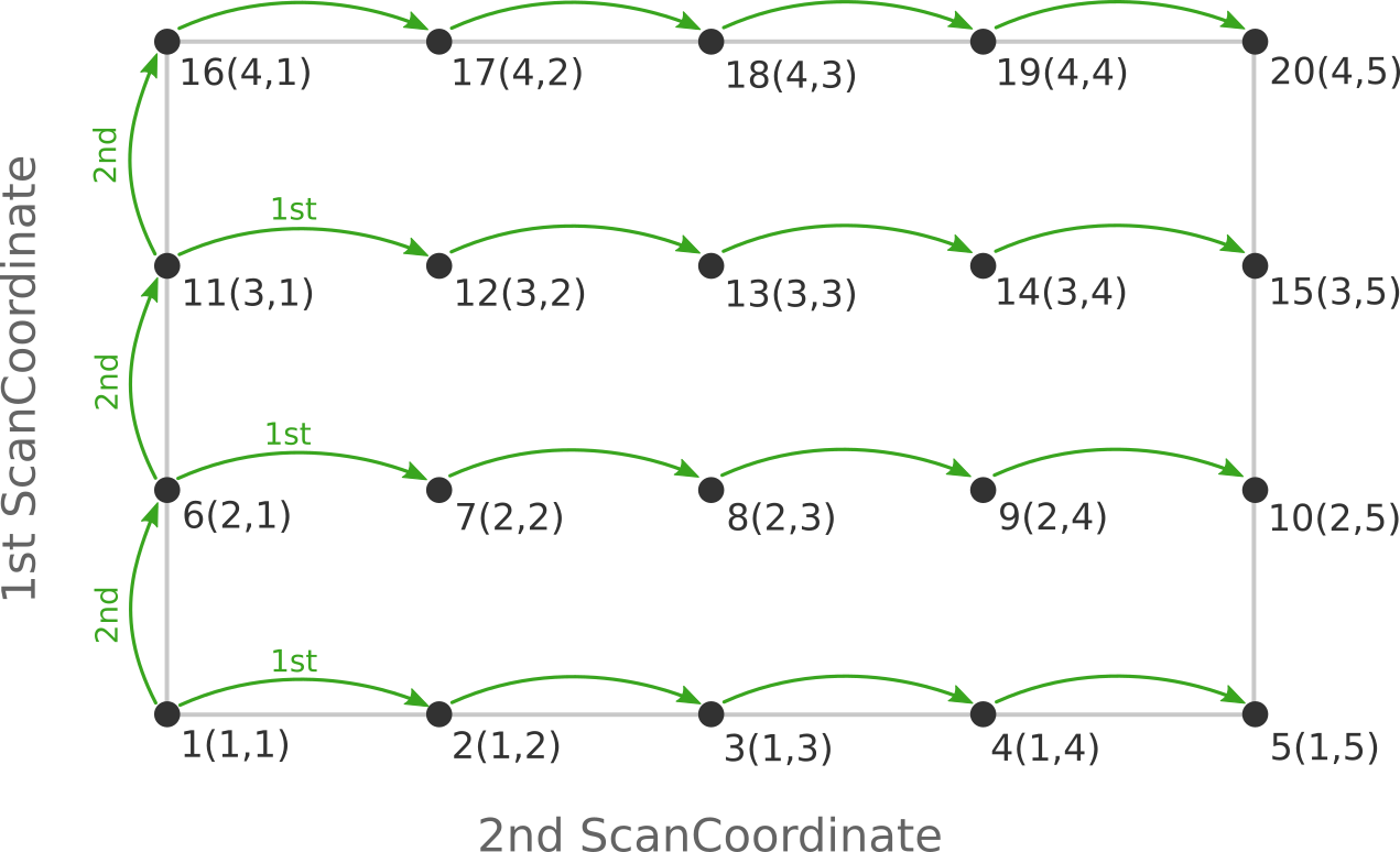
Here the scan starts at point 1(1,1) at the bottom left corner of the PES and first moves along the entire range of the 2nd scan coordinate, before taking a step along the 1st coordinate to point 6(2,1). The same PES points could be visited in a different order (and under different names) if the order of the two ScanCoordinate blocks is reversed in the AMS input:

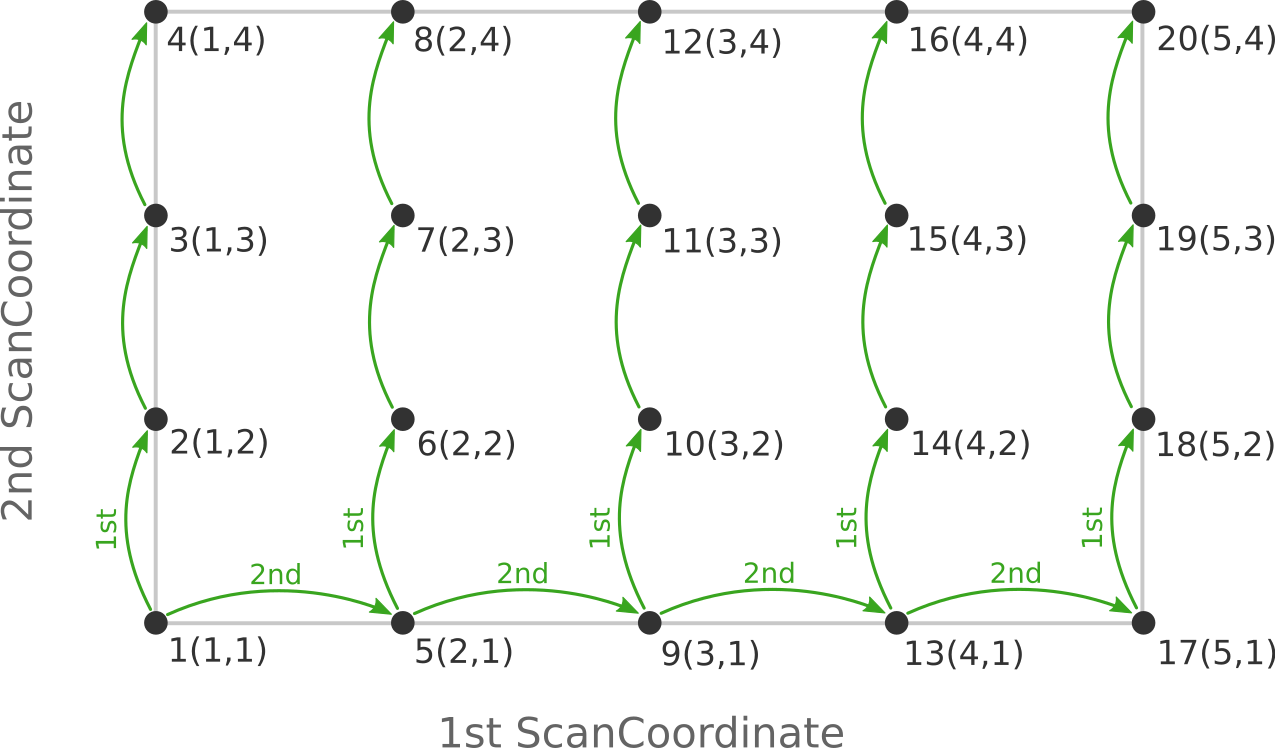
Depending on the shape of the scanned potential energy surface a particular order of visiting the PES points might be easier or harder for the optimizer, and convergence problems can sometimes be fixed by simply changing the order of the scanned coordinates. In the example above, it might be that scanning along the “vertical” direction is “harder” than scanning along the “horizontal” direction. In this case one should use the scan order from the first picture, which has only three “vertical” steps (whereas the other scan order has 15).

Note that AMS has a little safe-guard built in to help with PES scan convergence issues: If the optimization towards a particular PES point did not succeed in the initial attempt, AMS will later try again, but starting from a different (converged) point close to the unconverged one. This “PES gap filling” happens at the very end of the calculation, after the initial scan has been completed. This gap filling step is enabled by default, but can be controlled with the PESScan%FillUnconvergedGaps keyword:

PESScan

FillUnconvergedGaps

Type:

Bool

Default value:

Yes

Description:

After the initial pass over the PES, restart the unconverged points from converged neighboring points. This has no effect if the Optimize key is set to False.

Troubleshooting non-optimizing (rigid) PES scans¶

Rigid scans do not have geometry-optimizer convergence issues, but you may still see problems such as:

• Unexpected atoms moving: check bonding information. The moved fragment is determined from the bond graph.

• Rigid scan fails with an unsatisfied constraint error: the scan coordinate may not be compatible with a fragment-based internal coordinate change (e.g. for ring bond stretches).

• Atoms moving strangely in periodic systems: make sure the bonds involved in the scan coordinate do not cross the cell boundaries. (This case is not correctly implemented in AMS2026, but may be fixed in the future.)