Modeling Electrodeposition and Dendrite Growth

Note

To follow this tutorial, either:

• Download Electrodeposition.py (run as $AMSBIN/amspython Electrodeposition.py).

• Download Electrodeposition.ipynb (see also: how to install Jupyterlab)

Optionally:

• Download Electrodeposition-inlet.py.

• Download Electrodeposition-inlet.ipynb.

In battery engineering, controlling how metal grows at the microscopic level is a critical safety requirement. If electrodeposition is uneven, it can form sharp, needle-like dendrites that grow across the electrolyte and cause massive internal short circuits. Therefore, understanding and suppressing this dendrite formation is essential to preventing catastrophic battery failure.

In this tutorial, we will build a minimal kinetic Monte Carlo (KMC) model for metal electrodeposition using pyZacros. By explicitly simulating individual atomic events (such as ion diffusion in the electrolyte, electrochemical reduction at the interface, and surface self-diffusion on the electrode), we can visualize how macroscopic morphologies develop from the electrode.

Inspired by the work of Vishnugopi et al. Surface diffusion manifestation in electrodeposition of metal anodes Phys. Chem. Chem. Phys., 2020,22, 11286-11295, the core goal of this tutorial is to show how the competition between different surface diffusion pathways dictates whether a deposited film grows smooth and flat, or rough and fractal. Here we describe a simplified model. For surface diffusion, we will specifically include terrace diffusion and step-detachment (diffusion away from a step edge). By the end, you will have run a short simulation and visualized the direct link between atomic-scale kinetics and the resulting electrodeposition morphology.

OK, let’s start!

First, we import the main packages we need:

import scm.pyzacros as pz
import math

Next, we configure our environment for reproducibility and visualization. We set a deterministic random seed and import the matplotlib tools needed to visualize the simulation results.

import random

random_seed = 100
random.seed(random_seed)

%matplotlib inline
import matplotlib.pyplot as plt
import matplotlib.animation as animation

plt.rcParams["figure.figsize"] = [7, 7]

from IPython.display import HTML

Now, define a convenient set of physical constants:

kB = 8.6173e-05  # Boltzmann constant in eV/K
F = 96487.0  # Faraday constant in C/mol
R = 8.314  # Gas constant in J/mol/K
N_a = 6.022e23  # Avogadro constant in 1/mol

To reproduce these morphological changes, this tutorial will guide you through the complete setup of the pyZacros simulation. We will start from the ground up by defining the species and their energetic cluster expansions. With the physical entities established, we will build a 2D lattice and populate it with our initial electrode surface and electrolyte ions. From there, we will encode the actual physics (ion transport, reduction, and surface diffusion) into a network of elemental reactions. Finally, we will wrap these components into a ZacrosJob calculation, execute the KMC simulation, and animate the results to watch our metal deposit grow dynamically over time.

Species and Energetics (Clusters)

We first need to define the fundamental building blocks of our system. As shown in the diagram below, we allow each lattice site to take on one of three states: an empty site * (representing the background solvent), a solid deposited metal atom M, or a solvated metal cation M+.

s = pz.Species("*", denticity=1, kind=pz.Species.SURFACE)
M = pz.Species("M", denticity=1, kind=pz.Species.SURFACE, mass=1.0)
Mp = pz.Species("M+", denticity=1, kind=pz.Species.SURFACE, mass=1.0)

Next, we use Clusters to define the energetics of these species. To keep this model minimal, we will stick to one-site energetic terms for M and M+ and assign them a baseline energy of zero. We also intentionally omit lateral interactions. In pyZacros, this means our cluster expansion is simply a single site (s) occupied by either an M or M+ species.

M_cluster = pz.Cluster(label="M", site_types=["s"], species=[M])
Mp_cluster = pz.Cluster(label="Mp", site_types=["s"], species=[Mp])

The Lattice

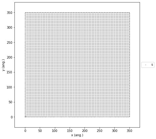
Our first step is to construct a 2D square lattice with nearest-neighbor connectivity. We set the distance between adjacent sites to 3.5 Å (\(a = 3.5\)), which corresponds to the atomic spacing of our metal electrode. The lattice has periodic boundary conditions along both axes. Following the reference paper, we map the liquid electrolyte onto this same crystalline structure. We capture the physical difference between the liquid and solid phases indirectly by assigning different kinetic rates to their respective diffusion mechanisms. For the simulation size, we intentionally chose a 100 x 100 grid. This specific scale strikes the perfect balance: it lets us track individual atomic hops while providing a large enough canvas to clearly see macroscopic features like nucleation density, growth front roughness, and island coalescence.

The code below creates this lattice and plots it so we can verify the setup is correct before moving on.

a = 3.5  # Lattice constant in ang

lattice = pz.Lattice(
    cell_vectors=[[a, 0.0], [0.0, a]],
    repeat_cell=[100, 100],
    site_types=["s"],
    site_coordinates=[[0.000000, 0.000000]],
    neighboring_structure=[[(0, 0), pz.Lattice.EAST], [(0, 0), pz.Lattice.NORTH]],
)

lattice.plot(marker_size=1, markers=["o"], colors=["0.8"]);

The Initial State

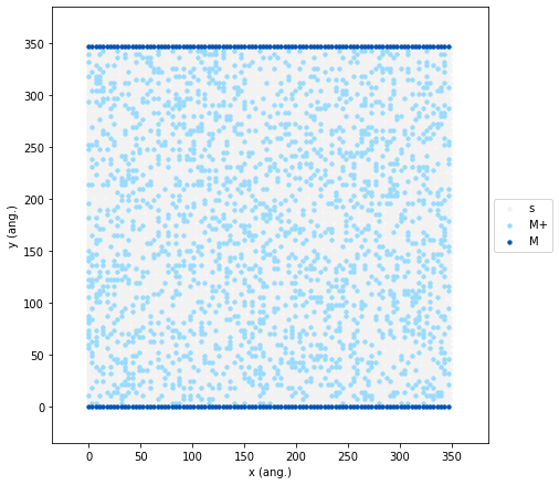
Once the lattice is built, we need to set up our initial “experimental” conditions. First, we create a Growth Front. We seed a horizontal line of M atoms along the bottom and top edges of the lattice. This acts as our initial conductive electrode surface where deposition will begin. Next, we add the electrolyte by randomly filling 20% of the remaining lattice sites with M+ ions. This specific 20% concentration provides a sufficient ionic flux to trigger visible competition between the two key processes, the rate at which ions reduce onto the surface, and the rate at which they diffuse along it.

initial_state = pz.LatticeState(lattice, [M, Mp, s], initial=True)

for sid in range(0, 100 * 100, 100):
    initial_state.fill_site(sid, M)
    initial_state.fill_site(sid - 1, M)

initial_state.fill_sites_random("s", Mp, 0.2)

0.2

To verify that our initial state is configured correctly, we can visualize it using the following code:

initial_state.plot(marker_size=2.5, markers=["o", "o"], colors=["#98dbff", "#0053b6"], lattice_color="0.95");

Elemental Reactions & Bulk Diffusion

The core of any KMC simulation is its reaction network. In our model, the electrodeposition dynamics are driven by four different elementary events:

1. Bulk Diffusion: M+ ions swap places with neighboring empty sites (*) to simulate random walk transport through the liquid electrolyte.

2. Electrochemical Reduction: An M+ ion adjacent to a solid M atom receives an electron and is reduced into a newly deposited M atom.

3. Surface Diffusion: Deposited M atoms hop across the surface. We explicitly track two pathways: terrace diffusion (moving along a flat plane) and step-detachment (moving away from a step edge).

4. Ion Replenishment: A background source term acts as an infinite reservoir, continuously introducing new M+ ions to maintain a steady concentration.

Now, let’s translate each of these physical steps into pyZacros elementary reactions.

Electrolyte Diffusion

First, let’s model how ions move through the liquid. We define ionic electrolyte diffusion as a reversible two-site hop where an solvated M+ ion swaps places with an adjacent empty site (*). On the left side of the image below, there is a representation of this process using graphs, as needed for pyZacros, which in this specific case consists of only two nodes. On the right side is the enumeration of the graph’s nodes. This graph is trivial, but it will be very useful later for more complex reactions.

Because diffusion in a liquid is faster compared to solid-state surface reactions, inputting raw physical rates introduces a computational “stiffness” problem into our KMC model. The solver would get bogged down simulating millions of fast ion hops without any actual deposition happening. To fix this, we apply a diffusion scaling factor (sf). This trick artificially slows down diffusion just enough to keep the simulation efficient, while maintaining the physical rule that bulk transport must remain at faster than the surface processes. For our setup, a scaling factor of 0.1 preserves this physical hierarchy.

We derive our diffusion coefficient from Valoen and Reimers J. Electrochem. Soc. 152 A882. Their fitted data for LiPF\(_6\) electrolytes suggests that at high concentrations (>4M, as in our case) and around 300 K, a reasonable order-of-magnitude estimate is \(D = 5 \cdot 10^{-7}\) cm\(^2\)/s.

Finally, when translating this into the pyZacros elementary reaction, notice that we set the activation energy to zero (activation_energy = 0). Because Zacros calculates rates using the Arrhenius equation, a zero activation barrier forces the exponential term to 1. This ensures that the prefactor we supply becomes equal to our rate constant.

D = 5.0e-7  # Diffusion coefficient of M+ in the electrolyte in cm^2/s
sf = 0.1  # Scaling diffusion factor
k_T = (D / a**2) * (1e16)  # Ion diffusion rate in 1/s

MpDiffusion = pz.ElementaryReaction(
    label="MpDiffusion",
    site_types=["s", "s"],
    initial=[Mp, s],
    final=[s, Mp],
    initial_entity_number=[0, 1],
    final_entity_number=[0, 1],
    neighboring=[(0, 1)],
    reversible=True,
    pre_expon=sf * k_T,
    pe_ratio=1.0,
    activation_energy=0.0,
)

Electrochemical Reduction

In this step, a local pair consisting of a solvated ion and a solid metal atom ([Mp, M]) transforms into two solid metal atoms ([M, M]). This represents the critical electron transfer event at the metal/electrolyte interface. Just as we did for bulk diffusion, the image below breaks down this process. On the left side, we see the graph representation of the physical reduction event. On the right side, we have the corresponding node enumeration.

We start by calculating the overall reaction current density (\(J\)) using the classic Butler-Volmer equation. You will likely recognize the standard experimental parameters used here, such as the applied overpotential (\(\eta\), eta), the exchange current density (\(i_0\)), and the operating temperature (\(T\)). However, pyZacros does not work with macroscopic currents, it requires a specific event frequency for a single atom! Therefore, we take \(J\) and scale it down to the area of just one lattice site (\(a^2\)). After applying standard unit conversions using Faraday’s constant (\(F\)) and Avogadro’s number (\(N_a\)), we finally arrive at \(k_R\), the per-site reaction rate in events per second. Finally, just as we did for bulk diffusion, we set activation_energy = 0, so our calculated \(k_R\) plugs directly in as the pre_expon parameter.

eta = 0.6  # Local overpotential in eV
i_0 = 5.0  # Exchange current density in mA/cm^2
alpha = 0.7  # Charge transfer coefficient alpha
beta = 1.0 - alpha  # Charge transfer coefficient beta
T = 300.0  # Operating temperature in K
J = i_0 * (
    math.exp(alpha * F * eta / R / T) - math.exp(-beta * F * eta / R / T)
)  # Faradaic reaction current density in mA/cm^2
k_R = J * a**2 * (N_a / F) * (1.0 / 1e3) * (1.0 / 1e16)  # Electrochemical reaction rate in 1/s

MpReduction = pz.ElementaryReaction(
    label="MpReduction",
    site_types=["s", "s"],
    initial=[Mp, M],
    final=[M, M],
    initial_entity_number=[0, 1],
    final_entity_number=[0, 1],
    neighboring=[(0, 1)],
    reversible=False,
    pre_expon=k_R,
    activation_energy=0.0,
)

Surface Diffusion

Once an atom is reduced onto the electrode, it does not necessarily stay where it landed. It can hop to neighboring sites. We model this surface self-diffusion using standard Arrhenius hopping rates:

\[k_T = \nu e^{-E_a / (k_B T)}\]

Here, \(\nu\) represents the attempt frequency—how often an atom vibrates and “tries” to jump to a new site (typically \(10^{12} - 10^{13}\) s\(^{-1}\)). For this example, we set \(\nu = 2 \cdot 10^{12}\) s\(^{-1}\) (nu)

nu = 2e12  # surface self-diffusion hopping frequency in 1/s

The activation barrier \(E_a\) will change depending on the local geometry of the hop. We use the values from the reference paper, but you can find inspiration on how to calculate such parameters from scratch using a quantum chemistry package (like the Amsterdam Modeling Suite) in this reference: Jäckle M. et al. Self-diffusion barriers: possible descriptors for dendrite growth in batteries? Energy Environ. Sci., 2018,11, 3400-3407.

To connect our model with the mechanistic discussion in the Vishnugopi et al. paper, we divide surface mobility into two distinct pathways.

1. Terrace diffusion: An atom hops laterally across a flat layer (intralayer hopping).

2. Diffusion away from a step: An atom escapes from a highly coordinated step-edge environment to a less coordinated site.

The original paper also studies a third pathway: interlayer (across-step) diffusion, where an atom descends from an upper terrace to a lower one. The authors identified this as the predominant mechanism for smoothing the surface and suppressing dendrites. To keep our tutorial model minimal and computationally fast, we have intentionally omitted this descending pathway.

First up is terrace diffusion. To implement this, we must translate the physical mechanism into a graph-based representation. The goal is to keep this representation as small as possible without losing the underlying physics (for instance, we need enough surrounding nodes to guarantee the atom is actually on a flat terrace and not perched on a step). The image below illustrates the diffusion process for our proposed graph representation and the corresponding node enumeration:

Based on the reference paper, we use \(E_a = 0.15\) eV for this reaction. The following code demonstrates how to translate the graph above into a pyZacros elementary reaction:

E_a1 = 0.15

MTerraceDiffusion = pz.ElementaryReaction(
    label="MTerraceDiffusion",
    #            0 ,  1 ,  2 ,  3 ,  4 ,  5 ,  6 ,  7
    site_types=["s", "s", "s", "s", "s", "s", "s", "s"],
    initial=[s, s, s, M, s, s, M, M],
    final=[s, s, s, s, M, s, M, M],
    neighboring=[(0, 1), (0, 3), (1, 4), (2, 3), (3, 4), (3, 6), (4, 5), (4, 7), (6, 7)],
    reversible=False,
    pre_expon=nu,
    activation_energy=E_a1,
)

Next, we define diffusion away from a step. Just as before, we translate this physical process into a graph. Notice that this specific mechanism requires a slightly larger 9-node cluster to properly capture the local geometry of the step and ensure the atom is moving away from it.

Following the reference paper, we assign this reaction an activation barrier of \(0.30\) eV. Notice that this is twice as high as the terrace diffusion barrier (\(0.15\) eV)! This energy penalty physically represents the difficulty of breaking the extra atomic bonds associated with a step-edge environment, capturing the reduced mobility of these trapped atoms.

Here is how we translate this graph into our final surface diffusion pyZacros reaction:

E_a2 = 0.30

MDiffusionAwayFromStep = pz.ElementaryReaction(
    label="MDiffusionAwayFromStep",
    #            0 ,  1 ,  2 ,  3 ,  4 ,  5 ,  6 ,  7 ,  8
    site_types=["s", "s", "s", "s", "s", "s", "s", "s", "s"],
    initial=[s, s, M, M, s, s, M, M, M],
    final=[s, s, M, s, M, s, M, M, M],
    neighboring=[(0, 1), (0, 3), (1, 4), (2, 3), (2, 6), (3, 4), (3, 7), (4, 5), (4, 8), (6, 7), (7, 8)],
    reversible=False,
    pre_expon=nu,
    activation_energy=E_a2,
)

Using a “Fictitious Gas” Strategy to Keep Ions Constant

To avoid the rapid depletion of M+ ions during deposition, we introduce a numerical replenishment event. We use a fictitious gas species (Mg) that continuously produces new M+ ions on empty sites at a constant rate \(k_A\).

Assuming a scenario where diffusion in the electrolyte is much faster than the interfacial reduction step, the ion addition rate should depend directly on the surface reduction rate

\[k_A=f_A k_R\]

Here, \(f_A\) can be physically interpreted as the probability fraction of having an M+ ion sitting directly against the electrode, ready to react. In practice, it serves as an empirical tuning parameter adjusted by trial and error to keep the overall ion concentration approximately constant. For our specific setup, we achieved this balance by setting \(f_A = 0.0005\).

The following code adds this fictitious gas species and the replenishment mechanism to our simulation:

Mg = pz.Species("Mg", gas_energy=0.0, mass=1.0)

f_A = 0.0005
k_A = f_A * k_R

MpAddIons = pz.ElementaryReaction(
    label="MpAddIons",
    site_types=["s"],
    initial=[s, Mg],
    final=[Mp],
    reversible=False,
    pre_expon=k_A,
    activation_energy=0.0,
)

Setting up the ZacrosJob and Running the Calculation

Now that we have all that we need, we are ready to configure the calculation. We do this using a Settings object, which controls the macroscopic conditions (temperature, pressure), simulation stopping criteria, and sampling time for different properties. Notice that we set the molar fraction of our fictitious gas (Mg) to 1.0. We also define an output sampling interval (\(\Delta t = 3 \cdot 10^{-8}\) s) to ensure we capture enough frames to properly resolve both the transient growth dynamics and the final surface morphology.

sett = pz.Settings()
sett.temperature = T
sett.pressure = 1.0
sett.molar_fraction.Mg = 1.0
sett.random_seed = random_seed

dt = 3e-8
sett.max_time = 15 * dt
sett.snapshots = ("time", dt)
sett.process_statistics = ("time", dt)
sett.species_numbers = ("time", 0.25 * dt)

Finally, we pack all components into a single ZacrosJob and execute it. Grab a coffee! On a typical laptop, this simulation should take about 20 minutes to complete!

cluster_expansion = [M_cluster, Mp_cluster]
mechanism = [MpDiffusion, MpReduction, MTerraceDiffusion, MDiffusionAwayFromStep, MpAddIons]

job = pz.ZacrosJob(
    settings=sett,
    lattice=lattice,
    mechanism=mechanism,
    cluster_expansion=cluster_expansion,
    initial_state=initial_state,
)

results = job.run()

[31.03|10:47:07] JOB plamsjob STARTED
[31.03|10:47:09] JOB plamsjob RUNNING
[31.03|11:06:04] JOB plamsjob FINISHED
[31.03|11:06:04] JOB plamsjob SUCCESSFUL

Analyzing the Results

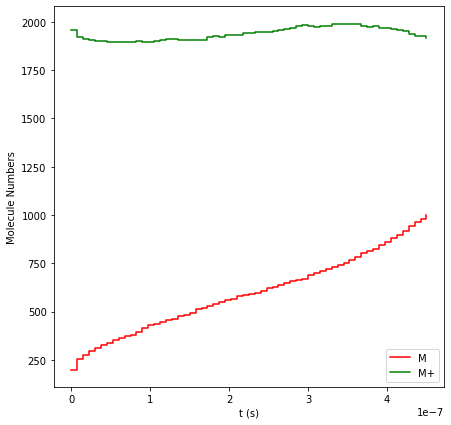
First, let’s look at how the species populations evolve over time. By plotting the molecule numbers, we can verify that our fictitious gas trick worked! The concentration of solvated M+ ions (the green line) remains approximately constant throughout the entire simulation. Notice the gradual deposition of solid M atoms (the red line), steadily growing from the initial seed surface up to a total of about 1000 atoms.

results.plot_molecule_numbers(["M", "M+"]);

To inspect the final spatial distribution of our deposited film, we can plot the last frame of the lattice_states trajectory (using index [-1]):

results.plot_lattice_states(
    results.lattice_states()[-1],
    marker_size=2.5,
    markers=["o", "o"],
    colors=["#98dbff", "#0053b6"],
    lattice_color="0.95",
);

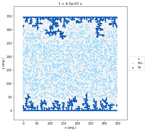
The resulting plot reveals the macroscopic morphology of the electrodeposited metal (M, dark blue). As expected from our kinetic parameters, the growth fronts have advanced inward from the boundaries, but the resulting deposit is highly uneven, exhibiting severe roughening and dendritic branching. This morphology is a direct consequence of our chosen reaction network. The fast electrochemical reduction rate outpaces the lateral surface diffusion (terrace diffusion and step-detachment). Furthermore, because we intentionally excluded interlayer (descending) diffusion from this minimal model, deposited atoms cannot easily relax into lower layers. This forces the system to grow outward into peaks and branches rather than forming a dense, conformal film.

As a final step, we can visualize the entire deposition process as a continuous animation. This dynamic view is often much more informative than a single final snapshot when trying to diagnose which kinetic step limits morphology evolution. The following cell uses matplotlib.animation.ArtistAnimation to compile our sequence of lattice states into a movie. We then use the to_jshtml() method to render an interactive HTML5 video player.

fig, ax = plt.subplots()

frames = []
results.plot_lattice_states(
    results.lattice_states(),
    show=False,
    marker_size=2.5,
    markers=["o", "o"],
    colors=["#98dbff", "#0053b6"],
    lattice_color="0.95",
    frames=frames,
)

ani = animation.ArtistAnimation(fig, frames, interval=500, blit=True)
plt.close(fig)  # prevent extra static figure display in notebook

HTML(ani.to_jshtml())

Once Loop Reflect

Controlling Morphology: The Low Overpotential Regime

You can easily alter the final morphology by shifting the kinetic balance of the simulation. If you adjust the initial parameters to a lower overpotential (eta = 0.4) and a longer time step (dt = 1e-6) to account for the slower reactions, the simulation will produce a dense, conformal film rather than dendritic branches.

Achieving this film-type deposition is the ultimate goal in metal anode engineering. A flat, uniform morphology minimizes localized current density “hot spots”, extends battery cycle life, and eliminates the safety hazards associated with dendrite-induced short circuits.

This shift in growth mode happens because lowering the overpotential exponentially decreases the rate of electrochemical reduction. With a much slower influx of new solid atoms, the system is no longer diffusion-limited. The deposited atoms have ample time to undergo lateral surface diffusion, allowing them to reorganize and relax into highly coordinated, tightly packed configurations before subsequent layers are formed.

The Inlet Model: Simulating Diffusion-Limited Growth (Optional)

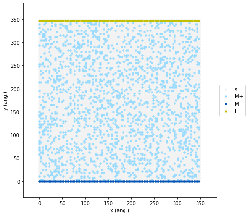
We can also model a system with a distinct concentration gradient by defining an explicit ion inlet rather than a uniform background reservoir.

In the code below, we define a new species I (Inlet). We initialize the lattice with our standard solid M electrode at the bottom (dark blue) and a solid line of I sites at the top (yellow). We also keep our initial 20% random seeding of M+ ions in the electrolyte solution.

I = pz.Species("I", denticity=1, kind=pz.Species.SURFACE, mass=1.0)
I_cluster = pz.Cluster(label="I", site_types=["s"], species=[I])

initial_state = pz.LatticeState(lattice, [M, Mp, s], initial=True)

for sid in range(0, 100 * 100, 100):
    initial_state.fill_site(sid, M)
    initial_state.fill_site(sid - 1, I)

initial_state.fill_sites_random("s", Mp, 0.2)

initial_state.plot(marker_size=2.5, markers=["o", "o", "o"], colors=["#98dbff", "#0053b6", "y"], lattice_color="0.95");

In this geometry, new M+ ions are continuously pumped into the system by the top yellow layer. This means they must physically diffuse across the entire simulation box to reach the bottom electrode before they can be reduced.

To implement this, we define a new elementary reaction where our fictitious Mg gas can only generate an M+ ion on an empty site (s) if it is directly adjacent to an Inlet site (I). Notice that we also increased our scaling fraction to f_A = 0.02. Because ions are now only entering the system from a single boundary row rather than uniformly across the whole grid, we need a higher local injection rate to maintain a steady overall flux.

Mg = pz.Species("Mg", gas_energy=0.0, mass=1.0)

f_A = 0.02
k_A = f_A * k_R

MpAddIons = pz.ElementaryReaction(
    label="MpAddIons",
    site_types=["s", "s"],
    initial=[I, s, Mg],
    final=[I, Mp],
    neighboring=[(0, 1)],
    reversible=False,
    pre_expon=k_A,
    activation_energy=0.0,
)

Finally, we update our cluster_expansion to include the new inlet species, our mechanism with the new MpAddIons reaction and execute the updated ZacrosJob. To ensure the injected M+ ions have enough time to diffuse from the top boundary down to the working electrode, we increased the time step by a factor of 4 (previously \(3\cdot 10^{-8}\) s), which indirectly increased the total simulation time. Perfect time for a lunch break! On a typical laptop, this calculation will take around an hour to wrap up.

cluster_expansion = [M_cluster, Mp_cluster, I_cluster]
mechanism = [MpDiffusion, MpReduction, MTerraceDiffusion, MDiffusionAwayFromStep, MpAddIons]

dt = 1.2e-7
sett.max_time = 15 * dt
sett.snapshots = ("time", dt)
sett.process_statistics = ("time", dt)
sett.species_numbers = ("time", 0.25 * dt)

job = pz.ZacrosJob(
    settings=sett,
    lattice=lattice,
    mechanism=mechanism,
    cluster_expansion=cluster_expansion,
    initial_state=initial_state,
)

results = job.run()

[31.03|11:10:31] JOB plamsjob STARTED
[31.03|11:10:33] JOB plamsjob RUNNING
[31.03|12:13:49] JOB plamsjob FINISHED
[31.03|12:13:49] JOB plamsjob SUCCESSFUL

We have successfully run our directional model! First, let’s take a look to the population numbers:

results.plot_molecule_numbers(["M", "M+"]);

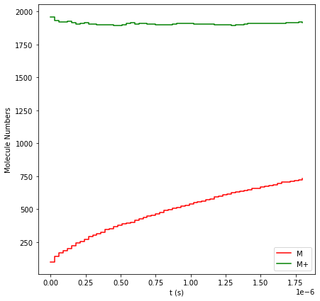
The green line shows that our new injection rate (f_A = 0.02) perfectly balances the reduction rate, keeping the overall M+ concentration steady while the solid M film grows.

Now, lets see the final spatial distribution of our deposited film:

results.plot_lattice_states(
    results.lattice_states()[-1],
    marker_size=2.5,
    markers=["o", "o", "o"],
    colors=["#98dbff", "#0053b6", "y"],
    lattice_color="0.95",
);

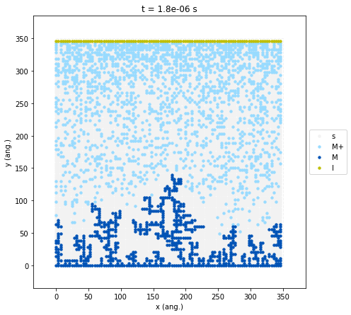
By introducing a physical distance between the ion source (the I inlet at the top) and the reduction surface (the electrode at the bottom), the simulation naturally develops a concentration gradient. The M+ species (light blue) is highly concentrated near the inlet but significantly depleted near the growth front. Furthermore, we can clearly observe localized depletion zones around the dendrite tips. This indicates a diffusion-limited growth regime. The highest peaks grow so fast that they consume all the nearby ions before those ions can travel down into the lower areas. Because the valleys are left “starved”, an even film cannot form, which just causes the dendrites to grow further out of control.

Now, just for fun, let’s create an animation to watch the dendritic morphology evolve over time!

fig, ax = plt.subplots()

frames = []
results.plot_lattice_states(
    results.lattice_states(),
    show=False,
    marker_size=2.5,
    markers=["o", "o", "o"],
    colors=["#98dbff", "#0053b6", "y"],
    lattice_color="0.95",
    frames=frames,
)

ani = animation.ArtistAnimation(fig, frames, interval=500, blit=True)
plt.close(fig)  # prevent extra static figure display in notebook

HTML(ani.to_jshtml())

Once Loop Reflect