The Ziff-Gulari-Barshad (ZGB) Model
In the previous tutorial, we have shown how the Zacros input files can be translated to pyZacros scripts. Here, we will show some additional examples for post-processing of the simulation output.
The example script can be downloaded through this link: ZiffGulariBarshad.py.
pyZacros Setup
pyZacros scripting can be used to immediately visualize the output of your simulation, enabling automated report generation. Various built-in functions are available to access commonly-used reports.
The basic structure of the script is much the same as in the preceding tutorial. We start by defining the species, lattice, reactions and simulation settings. The parameters used for the Ziff-Gulari-Barshad model can be found in the models overview.
We use the run() call to start the Zacros simulation. A results object is generated once the simulation completes. This results object gives us access to the simulation output within Python. For this example, we add a check to make sure that the job has finished without errors (job.ok) before proceeding with the analysis.
scm.pyzacros.init()
results = job.run()

if job.ok():
    # Post-processing & visualization
    results.plot_lattice_states(results.lattice_states())

scm.pyzacros.finish()
Using the plot_lattice_states function allows us to generate snapshots showing the transient evolution of the lattice during the kMC simulation.
Running the Simulation
We will now run the example script using Python. For default AMS installations:
$AMSBIN/amspython WaterGasShiftOnPt111.py
An overview of the simulation settings will be shown and the jobs starts running. Once the simulation has completed, a movie will play showing the transient evolution of the lattice.
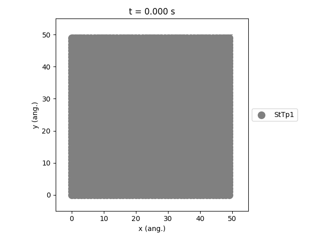
The StTp is the default name for a SiteType in Zacros. When constructing your own lattices, you can provide custom labels for the different sites, which will then also update the legend shown in the graph.
  1$ amspython ZiffGulariBarshad.py
  2[14.02|17:20:01] PLAMS working folder: /home/user/pyzacros/examples/ZiffGulariBarshad/plams_workdir
  3---------------------------------------------------------------------
  4simulation_input.dat
  5---------------------------------------------------------------------
  6random_seed         953129
  7temperature          500.0
  8pressure               1.0
  9
 10snapshots                 on time       0.5
 11process_statistics        on time       0.01
 12species_numbers           on time       0.01
 13max_time          25.0
 14
 15n_gas_species    3
 16gas_specs_names              CO           O2          CO2
 17gas_energies        0.00000e+00  0.00000e+00 -2.33700e+00
 18gas_molec_weights   2.79949e+01  3.19898e+01  4.39898e+01
 19gas_molar_fracs     4.50000e-01  5.50000e-01  0.00000e+00
 20
 21n_surf_species    2
 22surf_specs_names         CO*        O*
 23surf_specs_dent            1         1
 24
 25finish
 26---------------------------------------------------------------------
 27lattice_input.dat
 28---------------------------------------------------------------------
 29lattice default_choice
 30  rectangular_periodic 1.0 50 50
 31end_lattice
 32---------------------------------------------------------------------
 33energetics_input.dat
 34---------------------------------------------------------------------
 35energetics
 36
 37cluster CO*-0
 38  sites 1
 39  lattice_state
 40    1 CO* 1
 41  site_types 1
 42  graph_multiplicity 1
 43  cluster_eng -1.30000e+00
 44end_cluster
 45
 46cluster O*-0
 47  sites 1
 48  lattice_state
 49    1 O* 1
 50  site_types 1
 51  graph_multiplicity 1
 52  cluster_eng -2.30000e+00
 53end_cluster
 54
 55end_energetics
 56---------------------------------------------------------------------
 57mechanism_input.dat
 58---------------------------------------------------------------------
 59mechanism
 60
 61step *-0:CO-->CO*-0
 62  gas_reacs_prods CO -1
 63  sites 1
 64  initial
 65    1 * 1
 66  final
 67    1 CO* 1
 68  site_types 1
 69  pre_expon  1.00000e+01
 70  activ_eng  0.00000e+00
 71end_step
 72
 73step *_0-0,*_1-0:O2-->O*_0-0,O*_1-0;(0,1)
 74  gas_reacs_prods O2 -1
 75  sites 2
 76  neighboring 1-2
 77  initial
 78    1 * 1
 79    2 * 1
 80  final
 81    1 O* 1
 82    2 O* 1
 83  site_types 1 1
 84  pre_expon  2.50000e+00
 85  activ_eng  0.00000e+00
 86end_step
 87
 88step CO*_0-0,O*_1-0-->*_0-0,*_1-0:CO2;(0,1)
 89  gas_reacs_prods CO2 1
 90  sites 2
 91  neighboring 1-2
 92  initial
 93    1 CO* 1
 94    2 O* 1
 95  final
 96    1 * 1
 97    2 * 1
 98  site_types 1 1
 99  pre_expon  1.00000e+20
100  activ_eng  0.00000e+00
101end_step
102
103end_mechanism
104[14.02|17:29:40] JOB plamsjob STARTED
105[14.02|17:29:40] JOB plamsjob RUNNING
106[14.02|17:29:41] JOB plamsjob FINISHED
107[14.02|17:29:41] JOB plamsjob SUCCESSFUL
108[14.02|17:32:01] PLAMS run finished. Goodbye
Post-processing
In order to customize your own reports, you can simply add additional function calls to the post-processing block.
if job.ok():
    # Post-processing & visualization
    results.plot_molecule_numbers(["CO*", "O*"])
    results.plot_lattice_states(results.lattice_states())
Here, you can use any of the built-in visualization tools provided by pyZacros, or you can make your own analysis scripts by accessing the results data. (Examples for this are shown in the intermediate tutorials.)
pyZacros can also be used to load results from past jobs. This allows you to modify the visualization script without having to re-run the simulation.
job = pz.ZacrosJob.load_external( path="plams_workdir/plamsjob" )
job.results.plot_lattice_states(job.results.lattice_states())