Hyperfluorescence

Blue emitters, particularly those based on thermally activated delayed fluorescence (TADF), suffer from color impurity due to their broad emission spectra. The next generation hyperfluorescent emitters use a host-guest system with two types of emitters to obtain a narrower emission spectrum. The emitters in a hyperfluorescent OLED consist of a TADF sensitizer and a narrow-band fluorescent emitter. The TADF emitter reduces the losses associated with the generation of triplet excitons by converting triplets to singlets through reverse intersystem crossing (RISC). Instead of emitting radiatively after this process, the singlet excitons are transferred through Förster energy transfer (FRET) from the singlet state of the TADF emitter to the lower-energy singlet state of the narrow-band fluorescent emitter. The consequent radiative emission from the narrow-band fluorescent emitter then results in a narrower emission spectrum.

In this tutorial we will simulate a simple hyperfluorescence-based device as reported by Sachnik et al. [1]

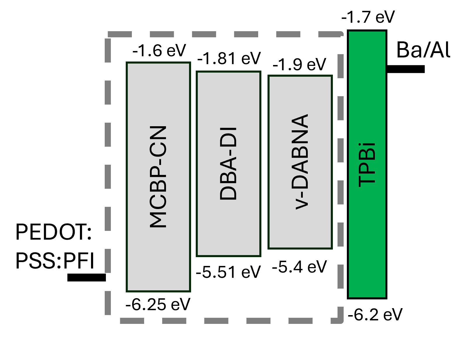
Fig. 121 The hyperfluorescent OLED stack, including HOMO and LUMO levels used as simulation input.

Note

A pre-made project file is available for this tutorial.

Create Materials

We start by importing our stack materials from the built-in database. Open BBinput and select the File → Import → Material option to access the database. Select the following materials:

• TPBi

• v-DABNA

• mCBP-CN

The parameters of these materials need to be adjusted to match the device reported by Sachnik et al. [1] (Due to differences in synthesis and evaporation conditions compared to the reference systems recorded for the database materials.) The material parameters can be adjusted by selecting the material and clicking on the pencil icon. The following input parameters will be changed:

TPBi

• Electronic

  • HOMO = -6.2 eV

  • LUMO = -1.7eV

  • Hole mobility prefactor = 0.5

  • Electron mobility prefactor = 0.5

• Excitonic

  • Singlet energy level = 3.75 eV

  • Triplet energy level = 3.5 eV

  • Tick the Link binding energies to energy levels box to automatically adjust the exciton binding energies.

  • Dexter prefactor (singlet) = 0.25

  • Dexter prefactor (triplet) = 0.25

v-DABNA

• Electronic

  • HOMO = -5.4 eV

  • LUMO = -1.9 eV

  • Hole mobility prefactor = 0.5

  • Electron mobility prefactor = 0.5

• Excitonic

  • Singlet energy level = 2.61 eV

  • Triplet energy level = 2.56 eV

  • Tick the Link binding energies to energy levels box to automatically adjust the exciton binding energies.

  • Dexter prefactor (singlet) = 0.25

  • Dexter prefactor (triplet) = 0.25

mCBP-CN

• Electronic

  • HOMO = -6.2 eV

  • LUMO = -1.7eV

  • Hole mobility prefactor = 0.5

  • Electron mobility prefactor = 0.5

• Excitonic

  • Singlet energy level = 3.75 eV

  • Triplet energy level = 3.5 eV

  • Tick the Link binding energies to energy levels box to automatically adjust the exciton binding energies.

  • Dexter prefactor (singlet) = 0.25

  • Dexter prefactor (triplet) = 0.25

Use the Save material button at the top of the page to save the updated material parameters.

Next, we define a new material for the TADF emitter DBA-DI. Click the button on the Materials page and select the TADF dye material template. The following input parameters are used:

DBA-DI

• Electronic

  • HOMO = -5.51 eV

  • LUMO = -1.81 eV

  • Hole mobility prefactor = 0.5

  • Electron mobility prefactor = 0.5

• Excitonic

  • Singlet energy level = 2.94 eV

  • Triplet energy level = 2.91 eV

  • Dexter prefactor (singlet) = 0.25

  • Dexter prefactor (triplet) = 0.25

Click the Save material button to save the input.

Create Compositions

In this tutorial we will be comparing two devices with a host-guest system containing different ratios of the host and guest materials. Navigate to the Compositions page and click the button. First, we define a 50% DBA-DI composition. Click the button to add materials to the composition. The material can be changed by double clicking the material name and selecting the desired material from the list. Similarly, the fraction in the composition can be adjusted as needed. For this tutorial we have set:

Material – Fraction

• mCBP-CN – 0.48

• DBA-DI – 0.5

• v-DABNA – 0.02

Save the composition with the Save composition button at the top of the page.

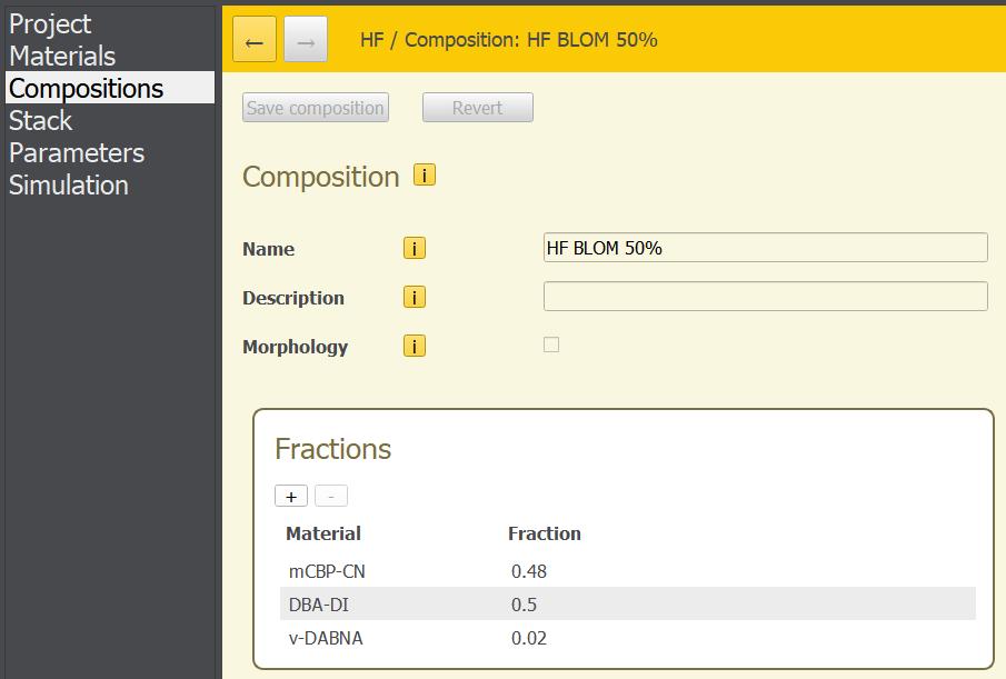
Fig. 122 Composition input for the 50% DBA-DI composition.

We also define a 25% DBA-DI composition as follows:

Material – Fraction

• mCBP-CN – 0.73

• DBA-DI – 0.25

• v-DABNA – 0.02

Create a Stack

Next, we will define the OLED stack on the Stack page. In the Layers section, add a layer of the 50% DBA-DI composition by clicking the button. Set the thickness to 82 nm. Then, add an additional TPBi layer and set the thickness to 3 nm.

Within the Förster interactions section, open the combinations dialog. Select all interactions and all materials under the Donors and Acceptors sections. Set the Förster radius to 2 nm and generate the interactions using the Generate button.

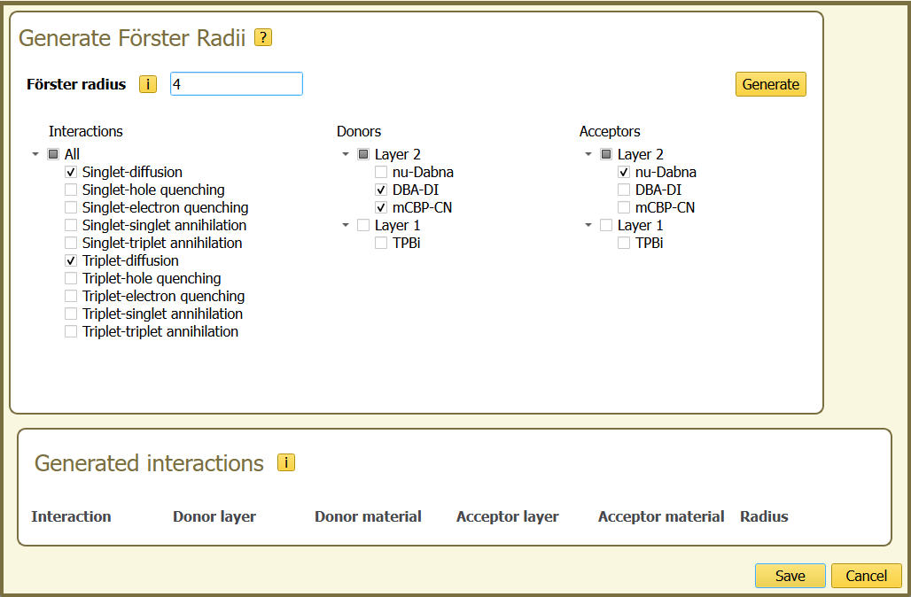
Fig. 123 The combinations dialog tab.

Next, enable both triplet and singlet diffusion under the Interactions section. In the Donors section, select mCBP-CN and DBA-DI, and in the Acceptors section, select v-DABNA. Set the Förster radius to 4 nm and generate the interactions. Save the interactions using the Save button in the bottom-right corner.

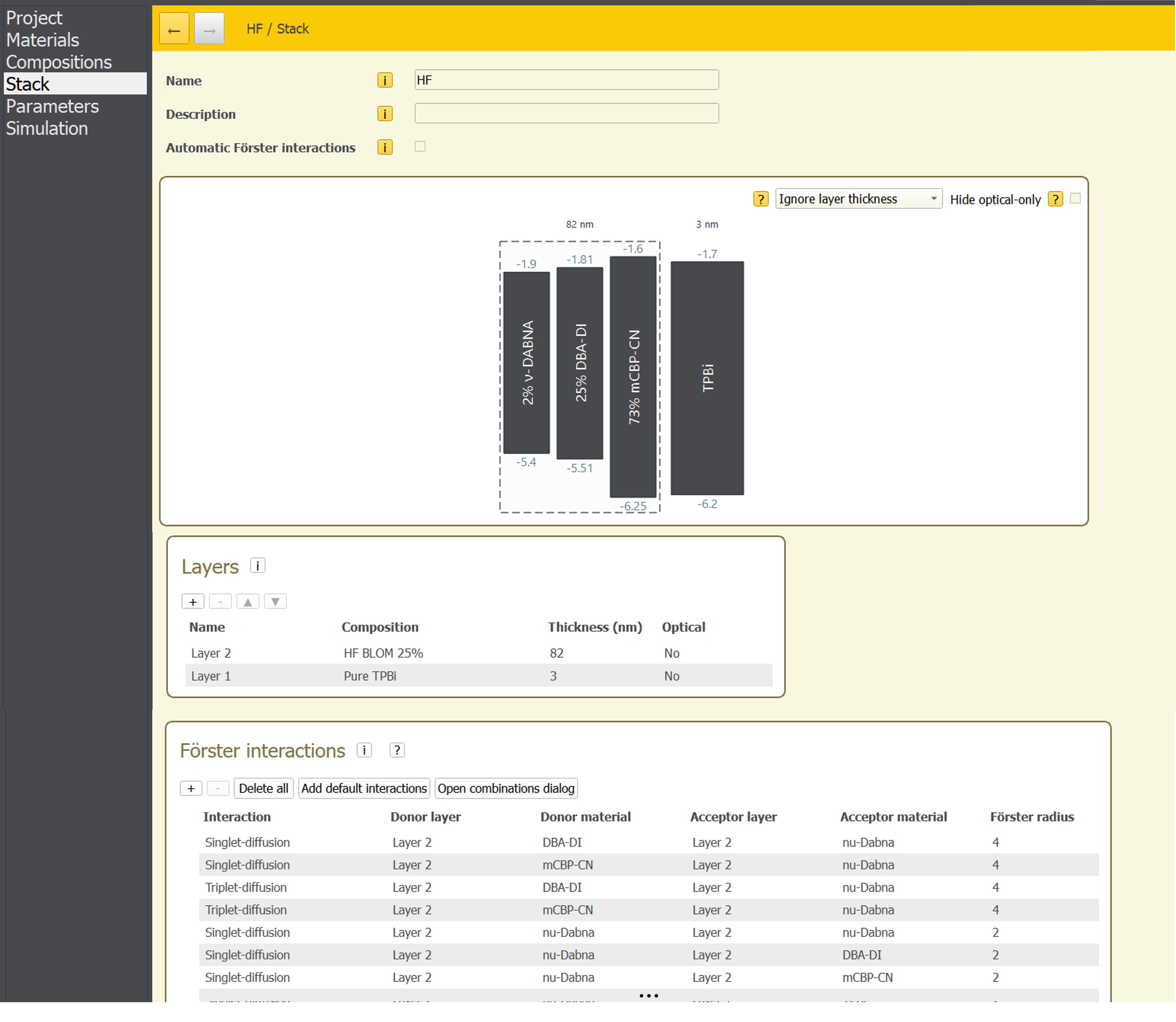
Fig. 124 The Stack input page, showing the layer input and the Förster interactions.

Create a Parameter Set

Navigate to the Parameters tab to configure the simulation parameters. Load the preset: Voltage sweep (bipolar). Adjust the Fermi level of the anode to -5.79 eV. (An Ohmic contact has been configured at the TPBi interface automatically.) Click the Save parameters button at the top of the page to save the input.

Start the Simulation

A voltage sweep can be configured in the Simulation tab. For this tutorial we set the following values:

• Trajectories

  • First trajectory = 0

  • Final trajectory = 3

• Sweep

  • Sweep parameter = voltage

  • From = 3 V

  • To = 5.5 V

  • Number of points = 6

After setting the parameters, save the simulation input for the 50% DBA-DI stack. Use File → Run to start the simulation.

Once the simulation has started, navigate back to the stack page and change the composition of the emissive layer to use 25% DBA-DI. Select Save stack to update the stack. We then use File → Save As and File → Run to create a new job for the 25% DBA-DI device.

Simulation Output

The simulation results can be monitored using BBresults.

J/V and luminance curves

The current-voltage and luminance characteristics can be found in the Device → Overview section. In the figure below, we compare the experimental and simulated J/V/L curves for both stacks. The simulated J/V and luminance curves of the 50% DBA-DI-based device show good agreement with the experimental data. Only a slight underestimation of the experimental values can be observed for lower voltages. The simulation of the device based on the 25% DBA-DI composition shows good agreement with the experimental values, with a slight overestimation at high voltage. This shows that Bumblebee is capable of accurately capturing differences in device functionality between two devices for the same simulation input.

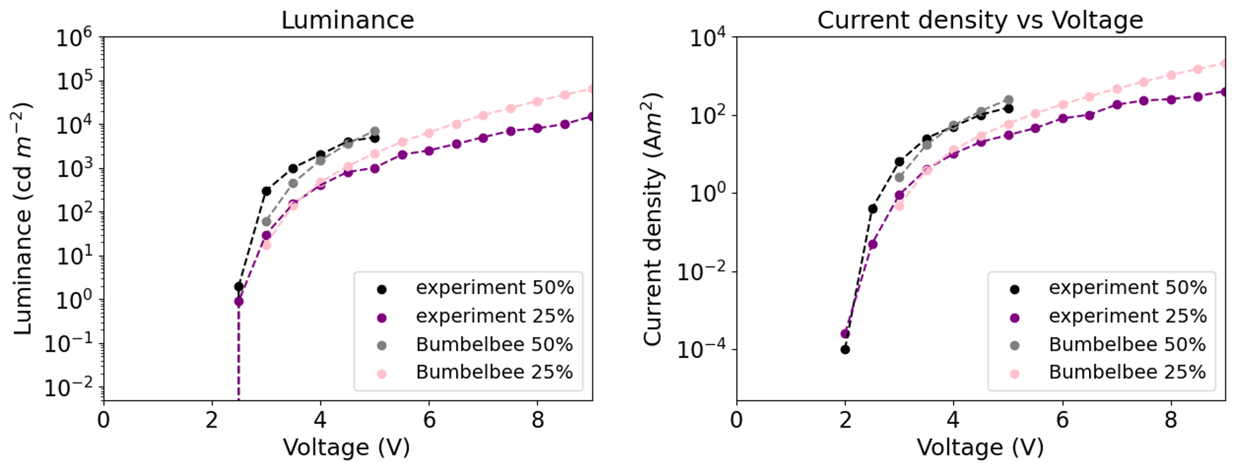
Fig. 125 Comparison of experimental and simulated J/V and luminance curves.

EQE

The external quantum efficiency (EQE) as estimated by Bumblebee for both devices is compared to the experimentally derived EQE. In the standard Bumblebee output, an optical outcoupling efficiency of 20% was assumed. Experimentally, outcoupling efficiencies are reported around 25%. The data in the figures below has therefore been scaled to match the experimental outcoupling.

Taking the outcoupling losses into account, the EQE determined for the 25% composition shows a good match with experimental data. The EQE of the 50% composition shows good agreement with the experimental data for higher current densities, but diverges for lower densities. Overall, we see relatively little change in the EQE. This trend is captured for both devices.

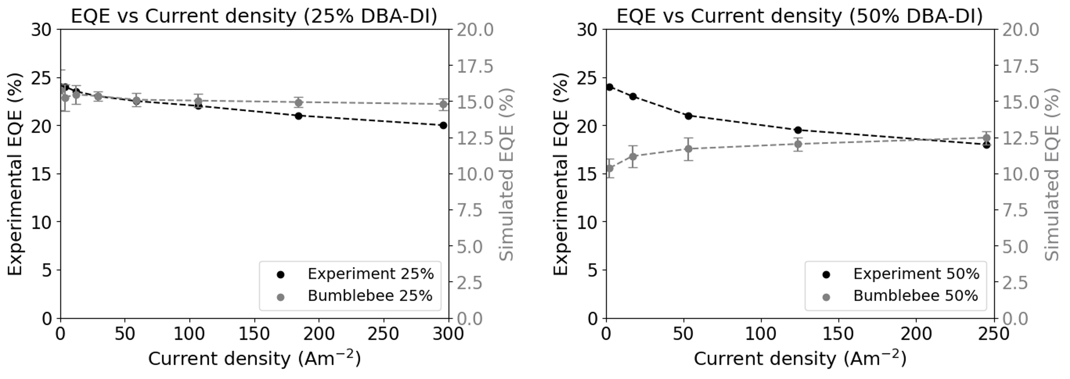
Fig. 126 Comparison of the experimental and simulated EQE for the 25% and 50% DBA-DI compositions.

Emission

The emission spectra can be found on the Sweep → Emission page in BBresults. For both devices, the maximum of the emission peak sits at 475 nm, in line with the emission wavelength of the hyperfluorescent emitter. The largest contribution of the emission spectra comes from v-DABNA, the narrow-band fluorescent emitter. A smaller peak, belonging to DBA-DI, the TADF emitter, can also be observed. The emission spectra show that the hyperfluorescence process is accurately reproduced by the configured FRET processes. While the TADF emitter can participate in emission, the exciton transfer process is preferred, resulting in the main emission peak belonging to v-DABNA, despite only making up 2% of the composition. This behavior is retained also at higher TADF fractions.

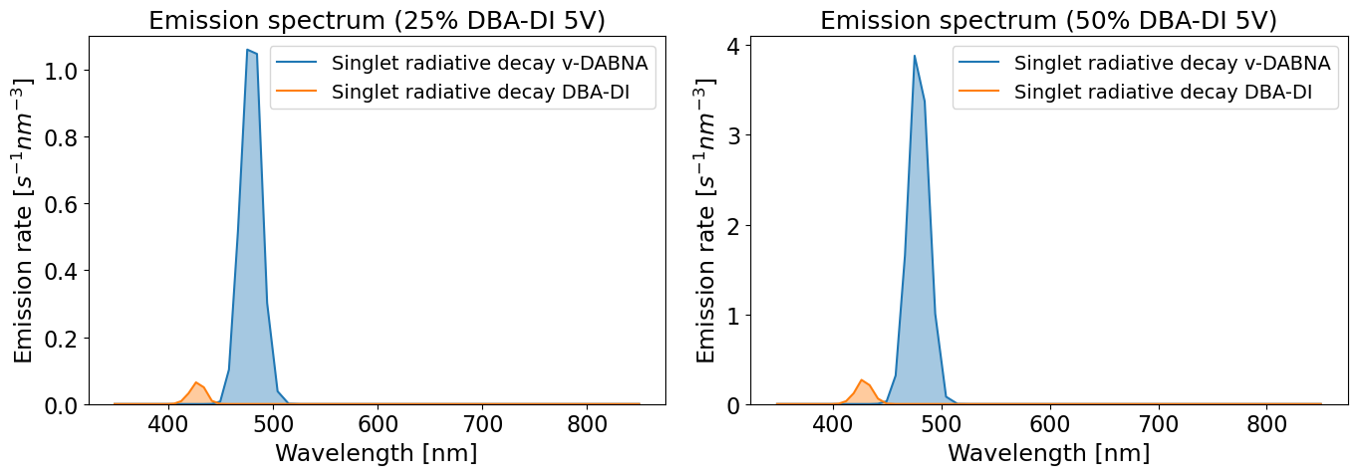
Fig. 127 The emission spectra of the 25% and 50% DBA-DI compositions.

References

[1] (1,2)

O. Sachnik, N. Kinaret, R. Saxena, M. Manz, W. Liu, J. Blaskovits, D. Andrienko, J. Michels, P. Blom, and G. Wetzelaer, * Pure-blue single-layer organic light-emitting diodes based on trap-free hyperfluorescence*, Nature Materials 11, 1742-1748 (2025).