Visualization of densities, orbital potentials, etc.

ADF AMSview Isosurface Contour lines Coulomb (electrostatic) potential

The AMSview module has many features. The basic use of AMSview is explained in the first tutorial.

In this tutorial, some additional features of AMSview are demonstrated using anthracene as a toy molecule:

Step 1: Get Single-Point calculation results with ADF on Anthracene

Start AMSinput

Set up an anthracene molecule (e.g. search for ‘anthracene’ in the search box and select the ‘Anthracene (ADF)’ molecule)

Run (File → Run) the calculation with all default settings

When the calculation has completed, open AMSview (SCM → View)

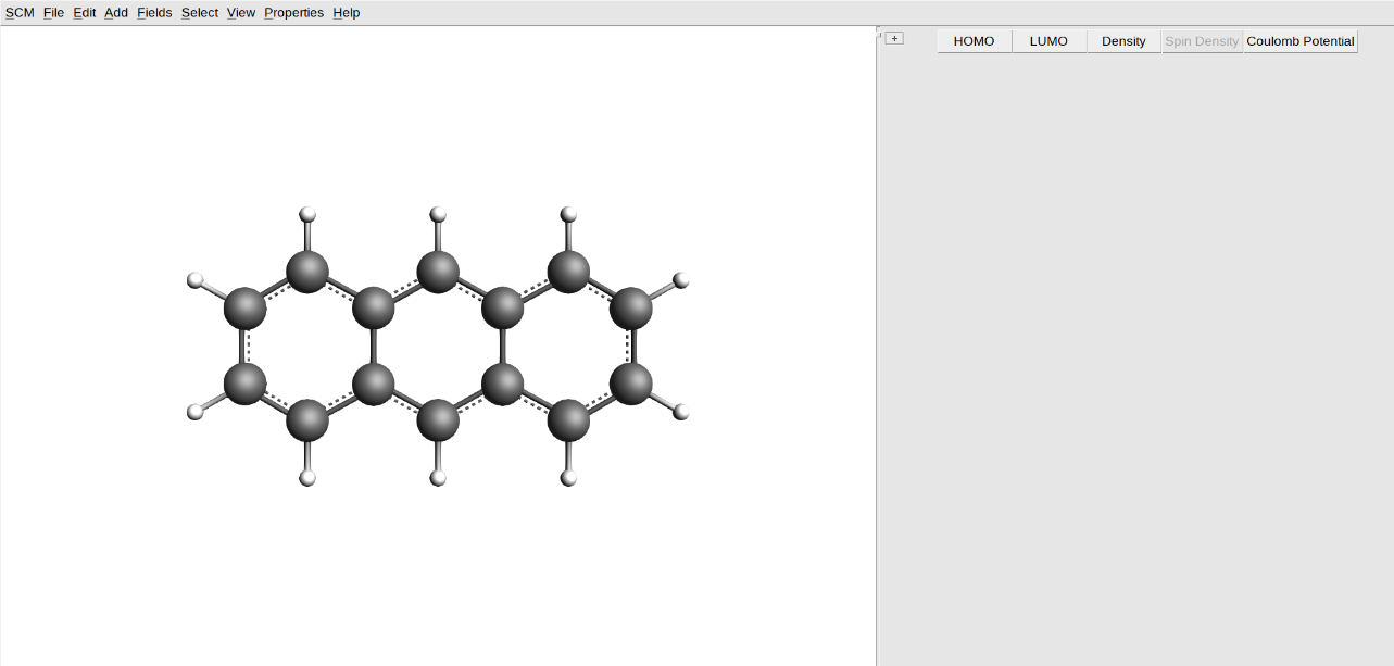
Step 2: Details: Diverging and Rainbow Colormap, scalar range of field on isosurface

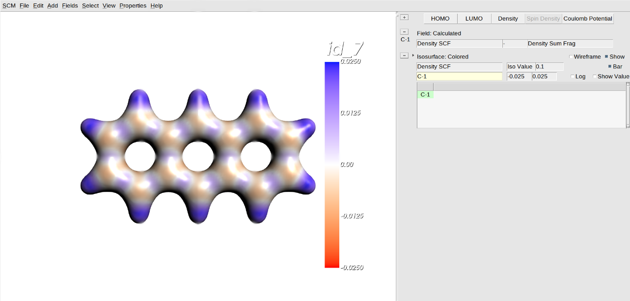
Now let’s generate an isosurface of the density colored by the electrostatic potential:

Add → Isosurface: Colored

In the Select Field… box in the new controls: Density → SCF

In the Select Color Field… box in the controls: Potential → Coulomb Potential SCF

Tick the Log box at the right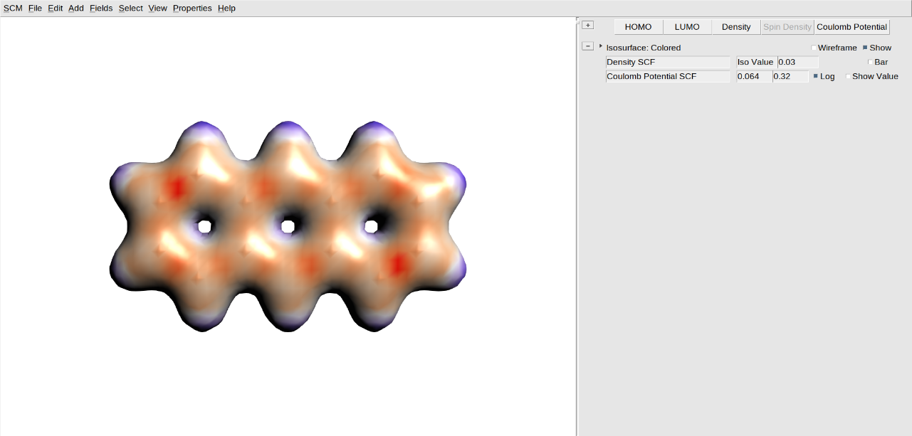

The image is not as smooth as it could be, because of the coarse grid used to calculate the density and potential. Improve it by using a better grid:

Fields → Grid → Medium

Click Yes to recalculate the 2 fields

Play around with the isovalue, and note how the two numbers on the right change

When you change the iso value, the default range for the coloring scheme is adjusted automatically (provided you have not changed it yourself). This range corresponds to the minimum and maximum value of the coloring field (in this case the SCF Potential) across the isosurface (in this case the SCF Density), at the isovalue you specify.

There is also an option to change the method used to interpret the given isovalue. The default “Normal” method uses the isovalue without modification. The “Contained” and “Squared” methods find the isosurface that contains the given percentage of the integrated field and integrated squared field, respectively. The “Volume” method finds the isosurface that matches the given percentage of the total grid volume.

Many more details can be set. First, begin by showing the color legend:

Check the Bar checkbox at the right

Click once in the color bar

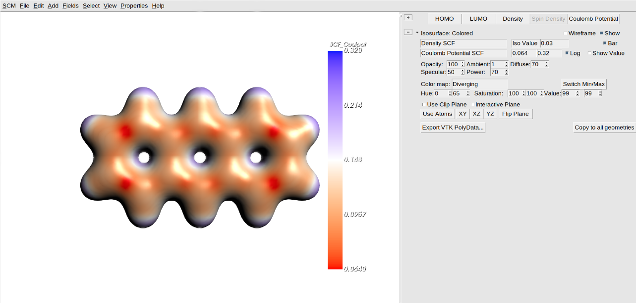
The color bar shows the mapping from colors to scalar values of the potential.

Clicking the color bar opens the detail controls.

Another way to open the details pane is to click the arrow on the left of the controls, in front of the visualization type (currently “Isosurface: Colored”).

The first part of the detailed controls allows you to adjust the appearance of the surface using settings like opacity, diffuse, specular, and power. Roughly speaking, these control how shiny or dull the surface looks and are referred to as the material properties controls.

The second part controls the color mapping. The Hue, Saturation, and Value fields allow you to specify two colors. The colormap option allows you to change how the transition from one color to the other works. The default colormap is Diverging: it goes from one pure color to white to the other pure color. Another colormap is Rainbow: it goes from one color to the other via other pure colors.

The third part allows you to control a clipping plane, cutting through the isosurface so you can look inside.

Select the Rainbow Colormap

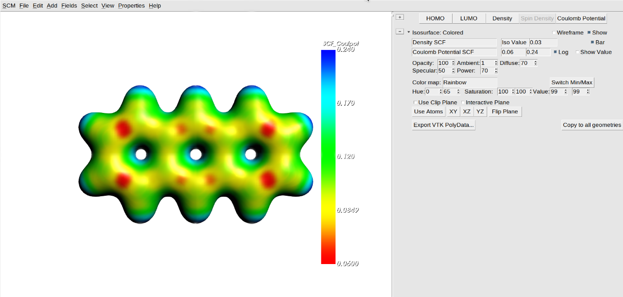
In general, the Diverging colormap makes it easier to see small variations in a property, although the Rainbow colormap is much more colorful. If you have a symmetric scalar range, the Diverging colormap puts the zero value at white. For the electrostatic potential this is not useful, but for a difference density it makes sense:

Delete the Colored Isosurface (use the left pull-down menu on that line)

Fields → Calculated

In the Calculated Field C-1 controls: select left field Density → SCF

In the Calculated Field C-1 controls: select right field Density → Density Sum Frag

Add → Isosurface: Colored

In the Colored Isosurface controls on the right-hand side: Left field selector: Density → SCF

In the Colored Isosurface controls on the right-hand side: Right field selector: Other → C-1

In the Colored Isosurface controls: change isovalue to 0.1

In the Colored Isosurface controls: show the color legend

In the Colored Isosurface controls: Specify a symmetric scalar range like -0.025 to 0.025

Step 3: Multiple Isosurfaces

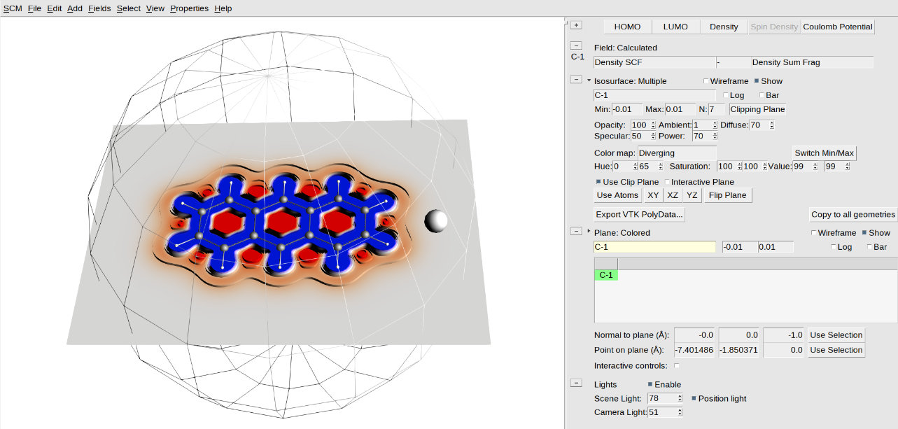
An even better way to see what happens to the density when forming a molecule from atomic fragments is the multiple-iso option. The idea is that a whole set of isosurfaces is generated for a range of iso values. The surfaces are colored by their isovalue.

In the Colored Isosurface line: Use the Delete command from the left pull-down menu

Add → Isosurface: Multiple

In the Multiple Isosurface line:

In the Select Field menu select the density difference: Other → 1 → C-1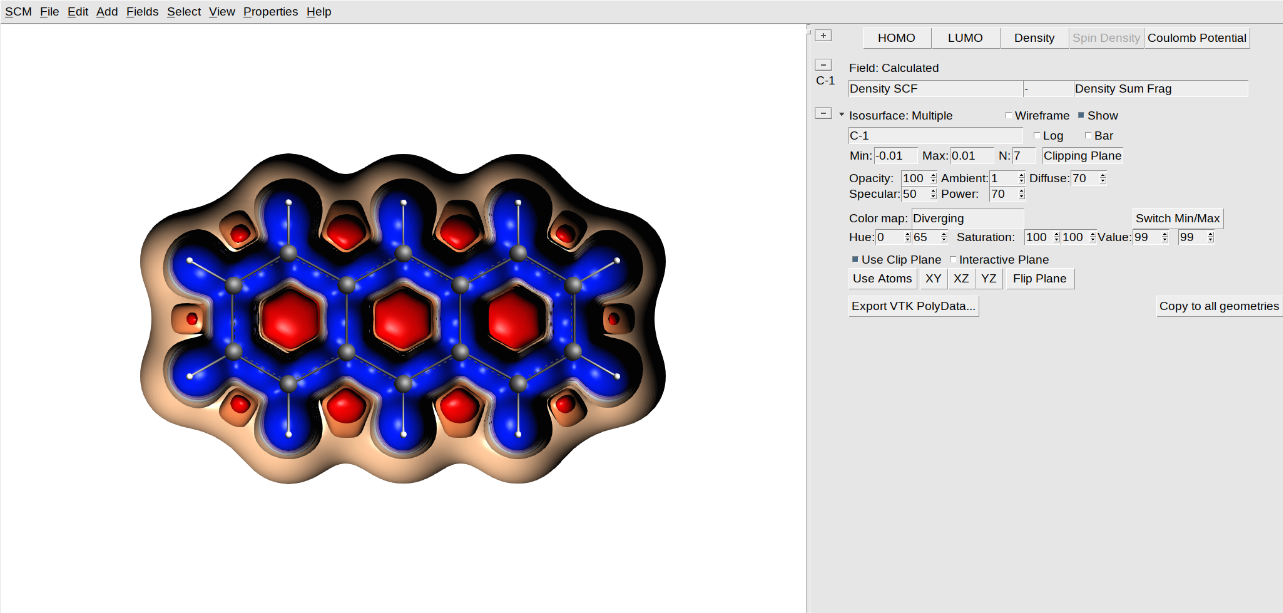

set N (the number of isosurfaces) to 7

change the min-max range to -0.01 … 0.01

Use Cmd/Ctrl + Minus repeatedly to make the atomic spheres very small

Fields → Grid → Fine

Click OK to confirm recalculating the fields

Rotate and zoom to get a good view

Now you can very clearly see that the electron density in the bonds is increased (blue), and where that electron density comes from (everywhere else, including close to the atoms).

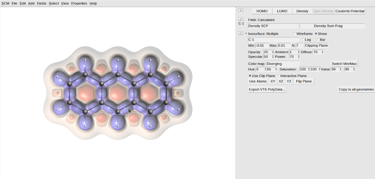
The clip plane allows you to cut away part of an isosurface, so you can look inside. The buttons on the last detail line allow you to position the clip plane as needed.

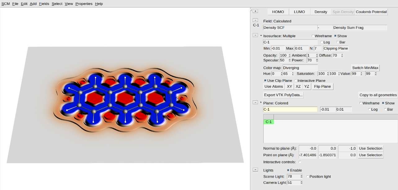
Instead of using a clipping plane, you can make the isosurfaces transparent:

Remove the clipping plane (uncheck the Use Clip Plane check box)

Change the Opacity to 20 %

View → View Direction → Along Z-axes

Zoom a little closer

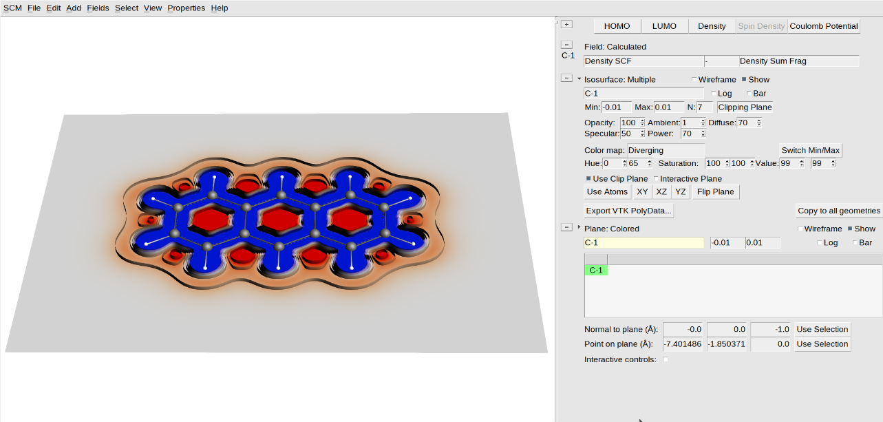
Step 4: Combining visualization techniques

You can also combine several visualization methods in one image.

In the Isosurface: Multiple controls, open the details and:

set Opacity to 100

rotate to look from the side

Check the “Interactive Plane” check box

Drag the red line to move the clipping plane slightly above the atom plane

(you might need to use the -XY button to realign it first)

Uncheck the “Interactive Plane” check box

Add → Plane: Colored

In the Plane: Colored controls:

Select the C-1 field

Select three atoms, and click the Position plane with atoms button

(note you can select atoms by shift-dragging a rectangle around an atom,

repeating this trick 3 times)

Use the same scalar range as for the Multiple Isosurface (without log option!)

Zoom to get a close view

Now you get a picture using the multiple-iso and colored-plane options at the same time.

Step 5: Play with lights

AMSview also has options to control lighting. This allows you to tune an image by adding a directed light source that casts shadows. You can also control the amount of ambient and directed light. It is hard in general to say what the best setting is, so try and play around:

View → Show Light Controls

In the extra light controls at the right side of the window:

Check the box to turn the light on

Check the box to position the light

Position the light as you like it

(you may have to rotate to be able to control the light properly)

Change the intensity of the extra light and the ambient light

(the Scene/Camera light controls)

Uncheck the box to position the light

Rotate and zoom as you prefer

One possible image you can make this way looks like this:

Step 6: Special fields

AMSview has access to a few fields that need extra clarification. One of these is the Steric Interaction, which uses the Van der Waals radius to visualize steric bulk. The field is the minimum distance to the Van der Waals surface of the selected atoms.

Delete the other surfaces present

Add an isosurface

Select a hydrogen atom

Select → Select Atoms Of Same Type

In the controls on the right-hand side, click Select Field… and choose Properties → Steric Interaction 1.

It is possible to make different selections and generate their own Steric Interaction field.