Combustion simulation (ReaxFF)

ReaxFF Oil & Gas PackMol Combustion Reaction network ChemTraYzer2 AMSmovie

In this tutorial we will set up a reactive MD simulation using ReaxFF for modeling the combustion of methane gas.

This tutorial will show you how to:

• Create a simple mixture (methane and oxygen)

• Set up a quick combustion reaction with ReaxFF

• Monitor and visualize the combustion process

• Analyze the reaction

Step 1: Start the GUI

Start AMSjobs

SCM → New input

Switch to ReaxFF: →

Set Periodicity → Bulk

Step 2: Create a methane / oxygen mixture

Next, we will make the methane / oxygen mixture. For full combustion, we need to have at least 2 oxygen molecules per methane molecule. To guarantee proper mixing, we choose to use a slightly leaner mixture with a CH₄:O₂ ratio of 1:2.5.

We will use the system builder in AMSinput to construct our mixture:

Builders → Packed Molecules Builder

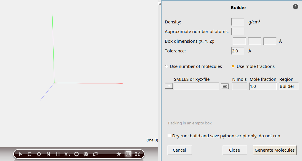
For this tutorial, we will focus on a high compression ratio with a gas density of 1.163 g/mL in order to encourage a fast combustion reaction.

Set Density to 1.163 g/cm³

Set Approximate number of atoms to 500

Tick Use mole fractions

Click the + button to add a second molecule to the builder

Click on the SMILES or xyz-file field of the first molecule

Type met to search for methane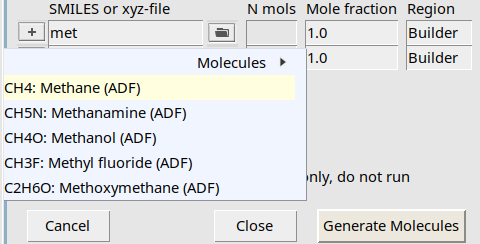

A list with search suggestions will appear, similar to the search box () in the panel bar.

Select Methane (ADF) from the search results

Set the mole fraction for methane to 1.0

Click on the SMILES or xyz-file field of the second molecule

Type o to search for O2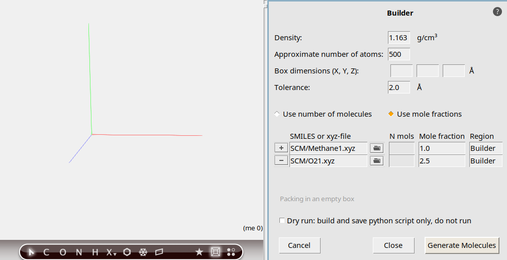

Select O2 (ADF) from the search results

Set the mole fraction for O2 to 2.5

We will now have the builder generate the molecules:

Click the Generate Molecules button

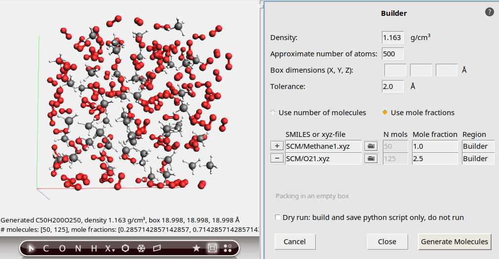
The molecules are generated at random non-overlapping positions and orientations. The output summary tells us the distribution of molecules in our mixture: 50 units of CH₄ and 125 units of O₂. This matches our description of the system, and we can now close the Builder menu.

Click the Close button at the bottom of the Builder window

Step 3: Set up the simulation

The next step is to set up the details of the simulation.

Note

For this tutorial, we will perform an MD simulation at both high temperature and density in order to make the combustion process proceed quickly. Typical scenarios using lower temperatures and/or densities will require longer simulation times in order to observe substantial conversion of reactants.

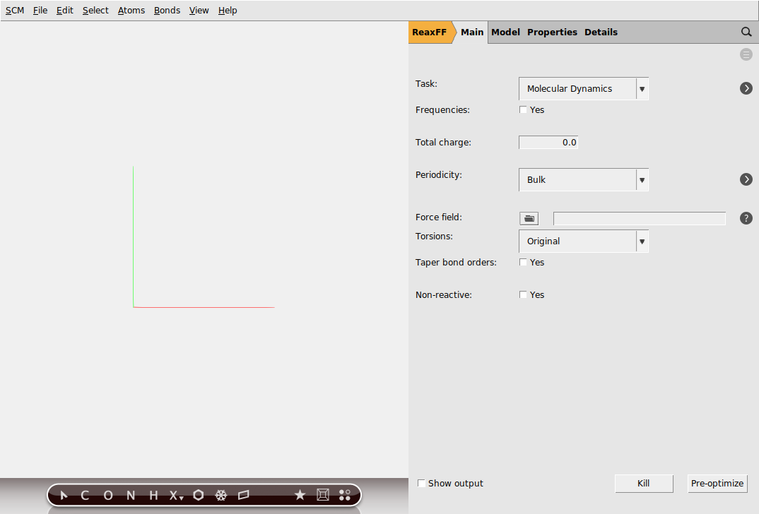
Click the next to the Force field entry in AMSinput

This will open a new window with a list of available force fields, including a short description of the relevant systems and references. For this particular example we will use the CHO force field for hydrocarbon oxidation.

Close the window describing the force fields

Click on the folder icon next to Force field

Select the CHO.ff force field

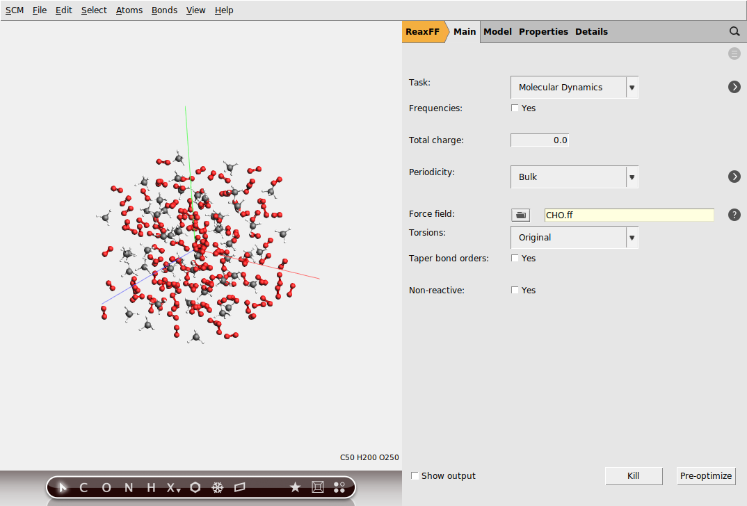
Next, we will configure the MD settings:

Click on next to Molecular Dynamics

Set the Number of steps to 30000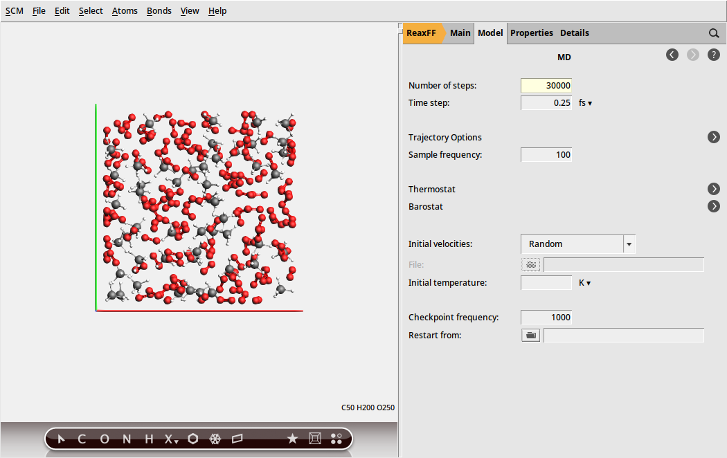

Note

In order to model a constant-temperature system (NVT), we apply a thermostat to the MD simulation. Because energy fluctuations may occur for reactive systems, we choose to use the Nose-Hoover thermostat.

The Nose-Hoover damping constant is dependent on the system size (as it effectively dampens the internal vibrations). For the current system, we use the default value of 100 fs.

When applying the combustion workflow to a realistic system, it may be worth testing different values to see which one yields the best performance.

To configure the Nose-Hoover thermostat:

Click on next to Thermostat

Click on the button to add a new thermostat

Select NHC from the Thermostat dropdown menu

Specify a Temperature of 3500 K and a Damping constant of 100 fs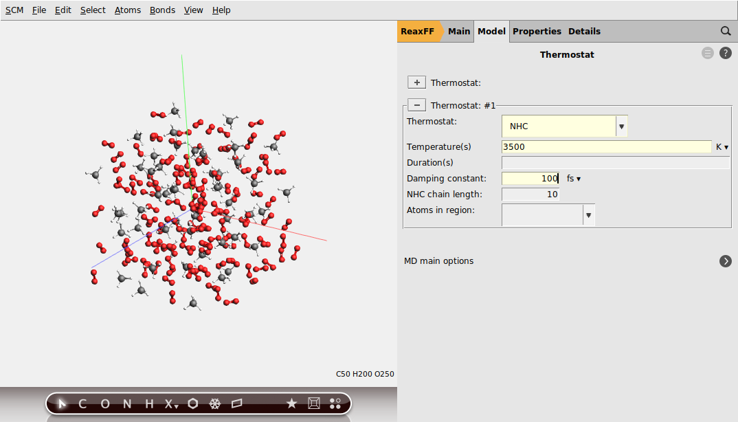

Step 4: Run the simulation

We will now run the combustion simulation.

Use the File → Run command

When asked to save your input, save it with the name Methane

Note

The simulation will take approximately 10 minutes. You can already proceed with the following steps while the job is running.

AMSjobs will come to the foreground, with the Methane job being shown at the top. Once the simulation starts, progress reports will be shown underneath the active job. We can also monitor the job output while the simulation is running:

Select the Methane job in AMSmovie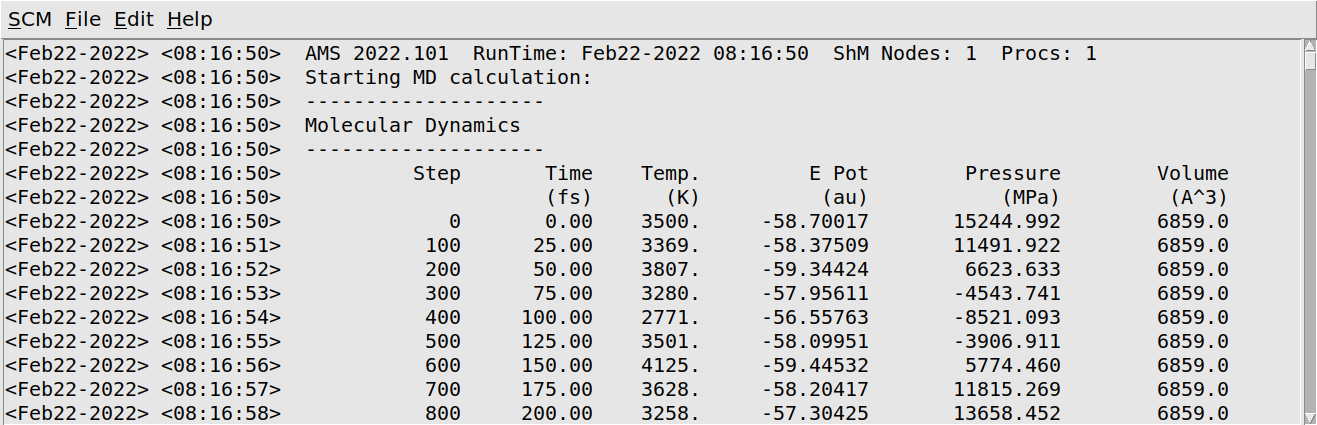

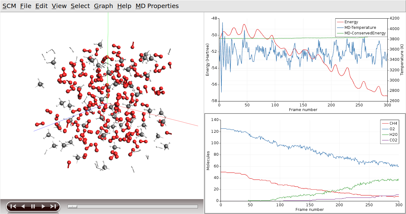
Click on SCM → Logfile to open the logfile

To see how the reaction progresses, we can visualize the output using AMSmovie. This works even while the simulation is still running:

Select SCM → Movie in the logfile window to open AMSmovie

Press the Play button (in the middle of the control panel, shown in the bottom-left corner of the AMSmovie window)

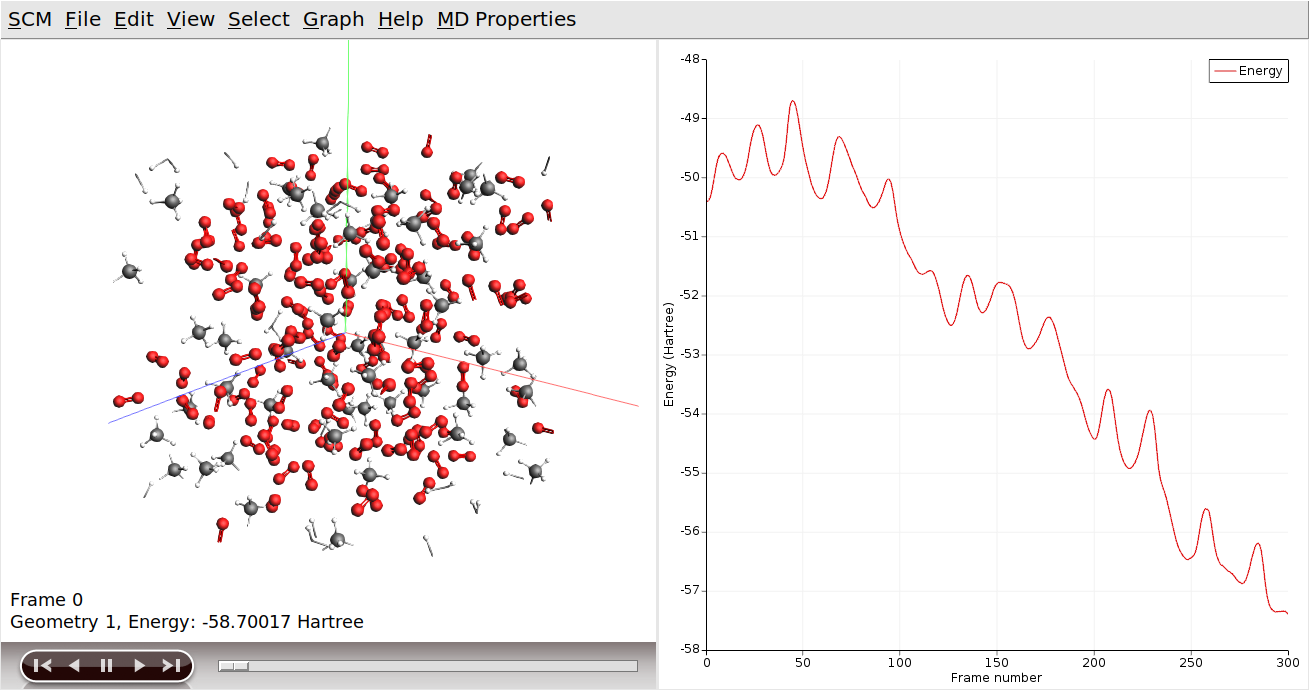
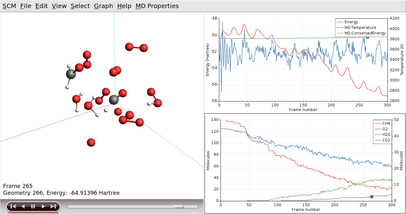
AMSmovie will show the molecular coordinates along the MD trajectory. New data is read in automatically as soon as it becomes available.

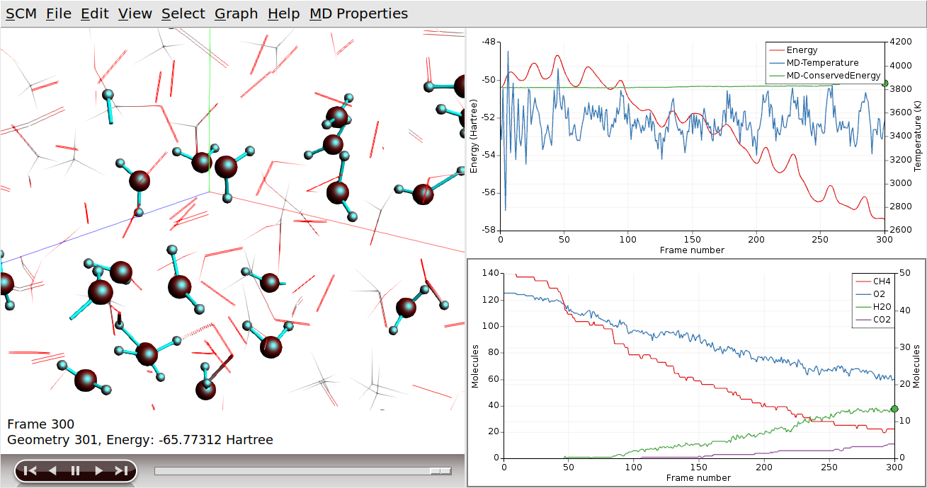
AMSmovie can also show graphs with some of the system properties that are calculated by ReaxFF:

In the AMSmovie window:

Use the MD Properties → Temperature command

Use the MD Properties → Conserved Energy command

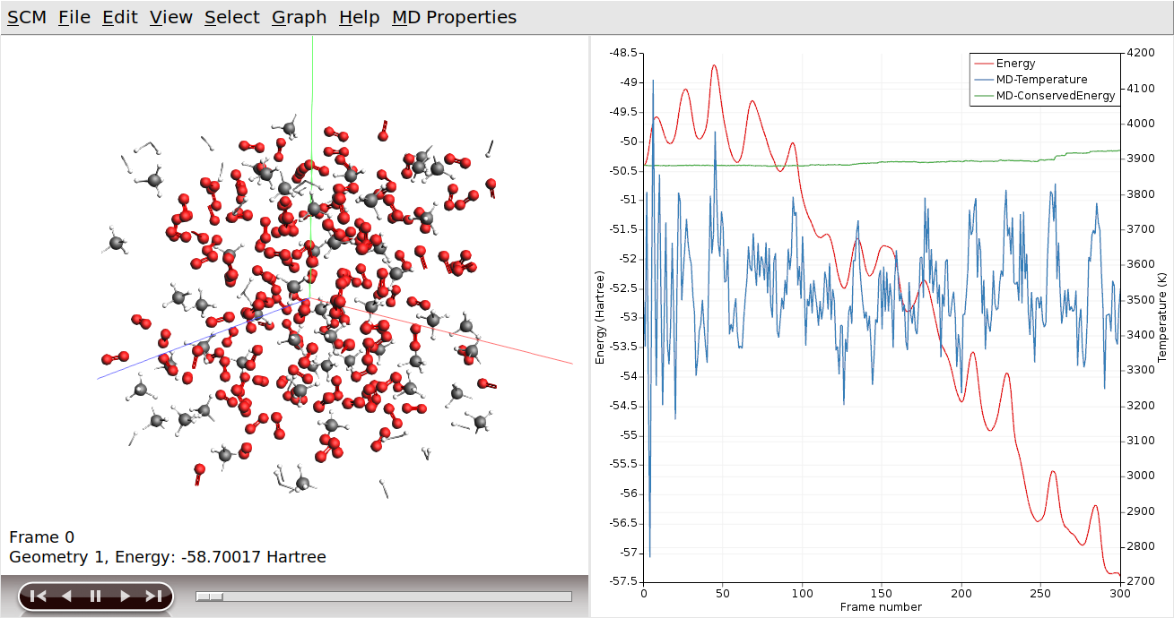
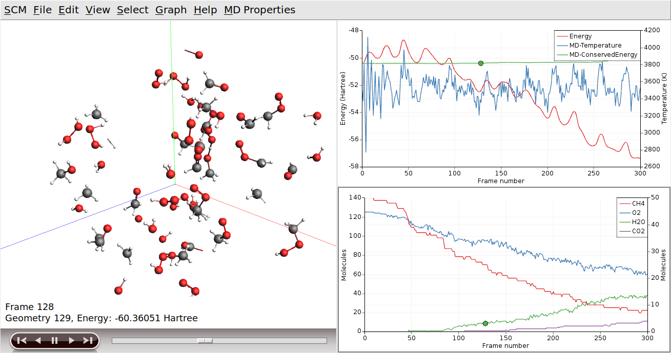
The slider at the bottom of the AMSmovie window can be used to move between different snapshots of the system. You can also click on a specific point in the graphs to pull up the corresponding state. The arrow keys (left and right) can then be used to move through the simulation one image at a time.

Tip

Jump to the end of the movie to automatically monitor the progress of the simulation

ReaxFF is a reactive force field, which allows reactions to take place during the MD simulation. In our example, methane and oxygen should react to form water and carbon dioxide. We can add graphs to show how many of the different molecule types are present at a given time:

After about 25000 iterations:

Use the MD Properties → Molecules… command

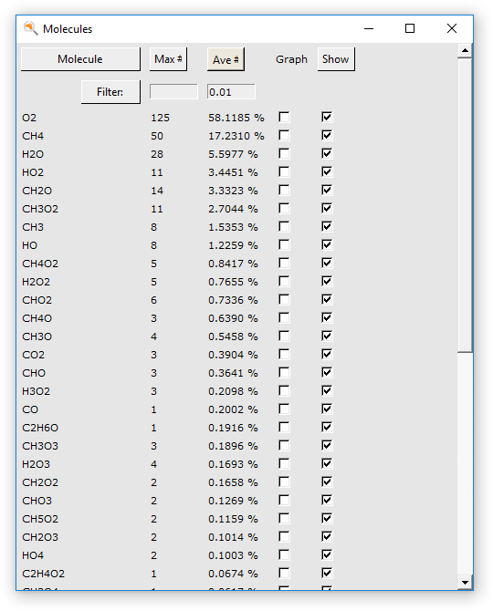
A dialog window will open, showing a list of the molecular species encountered during the simulation. The buttons at the top of the dialog allow sorting the molecules by name, occurrence in the last frame, or average occurrence.

Note

It may take a while before products are formed during the combustion simulation. Some reaction species may not appear in the Molecules menu if the simulation has not progressed far enough.

If this is the case here, you may need to wait a bit longer before new results come in. (Or in some cases, increase the total number of simulation steps.)

Note

The information shown in the Molecules dialog does not update automatically while the simulation is running.

You can refresh the list by closing and re-opening the dialog.

The first check box, labeled “Graph” is used to toggle the graphs for each of the molecular species. These graphs show how the number of molecules changes over time.

The second check box, labeled “Show”, allows you to hide molecules in the 3D model. This is convenient for e.g. monitoring product formation, or focusing on the distribution of specific reactants, as the other molecules can temporarily be hidden from view.

Two filter options are also included. These options hide species from the list for which either the number of occurrences or the mole fraction falls below the specified threshold. This is intended for more complex reaction systems, which can sometimes contain thousands of intermediate species.

Toggle the “Graph” check boxes for CH4, O2, H2O and CO2 (if present)

Tip

You can use the mouse to move the legends

Sometimes, it can help to put one of the curves on a different axis:

Click on the curve showing the number of CH4 molecules: this makes it the “active” curve

Use the Graph → Curve On Right Axes command

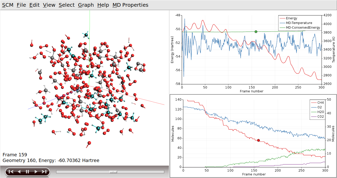
Clicking on the curve also had two other effects (besides making it the active curve): AMSmovie jumped to the snapshot matching the point where you clicked on the curve, and the corresponding molecules (CH4 in this case) are highlighted in the 3D view.

We can use the wireframe view to help make these molecules stand out from the rest:

Click an empty space in the 3D view so nothing is selected

Use the View → Molecule → Wireframe command

Click on the CO2 curve

Use the View → Molecule → Balls And Sticks to view the CO2 molecules more easily

Use the View → Fly To Selection command to focus the view

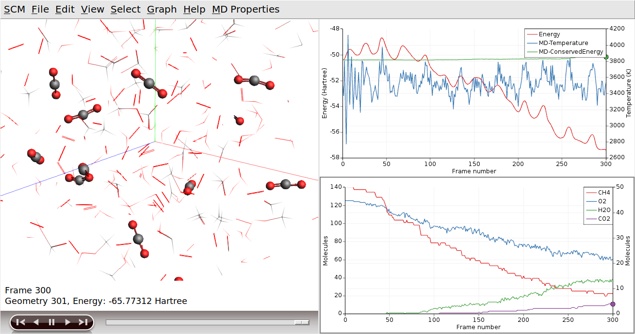
When moving through the movie, it is now easier to see how the reactions actually take place. (Note that atoms will remain selected, even if they are no longer part of a CO2 molecule.)

We can use the same procedure to focus on the H2O production:

Switch everything back to wireframe: View → Molecule → Wireframe

Click on the H2O curve

Use the View → Molecule → Balls And Sticks to view the H2O molecules more easily

Use the View → Fly To Selection command to focus the view

If we wanted to focus on both of our products at the same time, we can use the “Show” toggle in the Molecules dialog:

Clear the selection by clicking an empty space

Switch off the wireframe: View → Molecule → Balls and Sticks

Use the MD Properties → Molecules… command

Click on the “Show” check boxes for CH4 and O2 (they should now be unchecked)

Lastly, we can also focus in on a specific region of the simulation volume:

Select an atom somewhere in the center

Use the Select → Select Within Radius command

Set the distance to 5 Angstrom and choose OK

View → Show Selection Only

Click an empty space to clear the selection

View → Show All to see all the molecules again