VASP: TiO₂ surface relaxation

VASP Surface

This tutorial will teach you how to:

• Construct a slab for rutile TiO₂(001)

• Set up a geometry optimization job with constraints

• Set up a DFT+U VASP job to be run via the AMS driver

See also

Engine VASP documentation

Tip

• Download the GUI input file for this tutorial (optional)

Step 1: Check the VASP installation

Important

VASP is not distributed with the Amsterdam Modeling Suite. The VASP program must have been obtained and installed separately.

Verify that you have access to a working installation of VASP 5 or VASP 6, on either your local or a remote machine. If you want to run on a remote machine or computer cluster, check that you have set up a working AMSjobs queue for that system.

Check that you can run VASP. An example command could be:

mpirun -np 4 vasp # parallelize over 4 cores

Depending on your system, the VASP command may be called vasp_gam or vasp_std. If you do not know the proper command to launch VASP, ask your system administrator.

Step 2: Locate the POTCAR library

VASP requires the use of pseudopotentials or PAW potentials for each element. These are distributed with VASP in files called POTCAR or POTCAR.Z.

In this tutorial, you will use the Projector Augmented Wave (PAW) potentials for Ti and O constructed for the PBE density functional. You should have obtained those PAW potentials with VASP.

On your local machine (the machine running AMSinput), locate the needed POTCAR files. If you do not have them, you can download them from the VASP website.

For example, if the needed POTCAR or POTCAR.Z files are at

/some/path/PAW_PBE/Ti/POTCAR
/some/path/PAW_PBE/O/POTCAR

then the path /some/path/PAW_PBE/ would be the POTCAR Library that you need to specify in AMSinput.

See the POTCAR documentation for the VASP engine for more details.

Tip

Consider saving your VASP command and POTCAR library as a preset (Right click any input field → Save Preset VASP). The next time you open AMSinput and select the VASP engine, this command and POTCAR library will be used.

Step 3: Create the TiO₂(001) slab

1. Start AMSinput

2. Switch to VASP: →

3. In the menu bar, select Builders → Crystal Structure → Tetragonal → Rutile

4. Click OK to get the experimental rutile TiO₂ crystal structure unit cell (a = 4.59 Å, c = 2.96 Å).

Note

One would normally perform a lattice optimization of the bulk structure before creating a slab. In this tutorial, we will instead use the experimental lattice parameters.

Next, we create a 2-layer (001) slab. (Because the crystal unit cell contains 2 atomic layers, the resulting slab will actually be 4 atomic layers thick).

5. Select Edit → Crystal → Generate slab

6. Enter (0, 0, 1) as the Miller indices.

7. The number of layers should be set to 2 (default).

8. Click “Generate slab”.

9. Close the slab builder.

This should create a 2-layer slab in the 3D area on the left. Select View → View Direction → Along X-axis from the menu bar, or rotate the system so that the z-axis (shown as a blue line) is roughly displayed vertically. This will give you a side view of the slab.

Note

• It may happen that bonds are drawn between adjacent Ti ions. These bonds do not affect the VASP calculation and can safely be ignored.

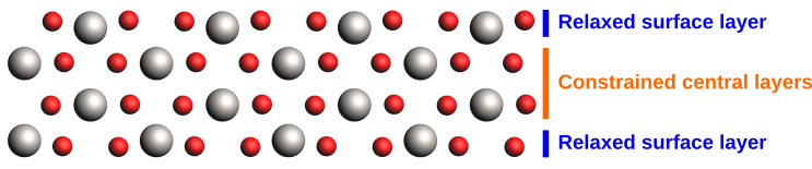
• A realistic slab model would typically require additional layers, such that the relaxation of the surface does not affect the bulk structure in the center of the slab. We will instead use geometry constraints here to reduce the size of our model.

All VASP calculations are performed under 3D periodic boundary conditions. Therefore, slabs are necessarily separated by a vacuum gap in the surface normal direction.

10. Click on the Periodic View Tool to visualize a few periodically repeated images of the central cell.

Note that the default vacuum gap is quite large. Because VASP uses a plane wave basis set, a large vacuum gap will increase the computational cost. For this reason, one typically wants to reduce the size of the vacuum gap as much as possible, while still keeping the periodic images from interacting with one another. For this tutorial, we will use a small vacuum gap of around 8 Å.

11. In the panel bar, select Model → Lattice.

12. Set the components of the c lattice vector to 0.0 0.0 14.0. (Note: this c lattice vector now refers to the slab system including the vacuum gap, and no longer to the original unit cell of the crystal).

13. Click on one of the Ti atoms in the center of the slab to select it. Then, in the menu bar select Edit → Crystal → Set (0.5, 0.5, 0.5). This moves the slab to the center of the vacuum gap, to make visualization easier.

14. Click again on the Periodic View Tool so that only a single periodic image is displayed.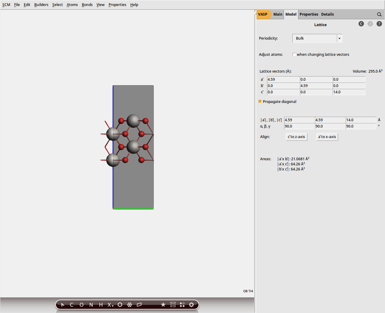

15. In the menu bar, select Edit → Crystal → Map atoms to (0..1). This places all of the atoms inside the displayed unit cell.

Note

Proper procedure is to systematically vary the vacuum gap for the particular system at hand. Calculated quantities (such as the surface energy, adsorption energies, work function, etc.) should converge as the vacuum gap is increased. One can then select the smallest vacuum gap while still obtaining converged values.

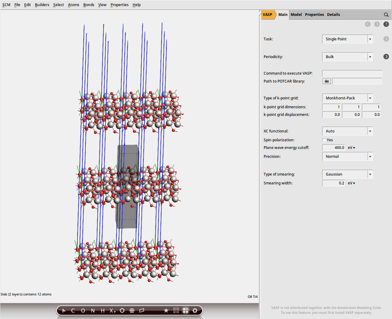
Step 4: Set the VASP settings

1. In the panel bar, select Main.

2. In Command to execute VASP enter the command from Step 1.

3. In POTCAR library enter the path to the PBE PAW POTCAR library from Step 2. This path will be remembered the next time you start AMSinput.

4. In the main panel, set the Type of k-point grid to Monkhorst-Pack (default).

5. Set the k-point grid dimensions to 3 3 1.

6. Set the XC functional to PBE.

7. Set the Plane wave energy cutoff to 400 eV (default).

8. Set the Type of smearing to Gaussian (default).

9. Set the Smearing width to 0.1 eV.

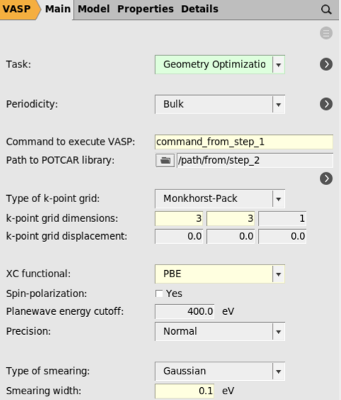
Note

The k-point grid dimensions and plane wave energy cutoff would normally be obtained through convergence tests.

10. In the panel bar, select Model → Hubbard U.

11. Check the Use DFT+U checkbox.

12. Set Hubbard U-type to 2 (default, the method by Dudarev et al.)

13. Set LMAXMIX to 4.

14. For Ti, set U to 3.0 eV, and l to d.

15. For O, set l to Disable.

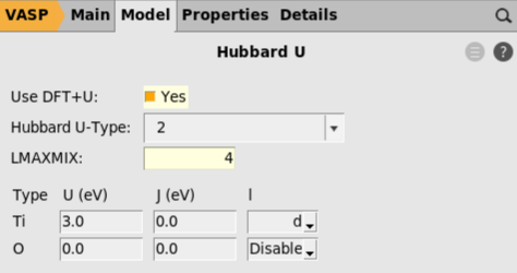
The main VASP input file, INCAR, contains a large number of settings for modifying technical aspects of the calculations. AMSinput does not provide dedicated panels for all of these options. Instead, the user is allowed to add specific settings to the INCAR directly. To illustrate this, we will modify the self-consistent-field algorithm.

16. In the panel bar, select Details → Expert VASP.

17. Type ALGO = Fast in the Additional INCAR options text box.

Step 5: Set the AMS settings

We will use constraints to restrict the geometry relaxation to the surface layers.

1. In the Main panel, select Task → Geometry Optimization.

2. In the panel bar, select Model → Geometry Constraints and PES Scan.

3. In the molecule drawing area, select the six atoms (2 Ti and 4 O) in the center of the slab. (Hold Shift to select multiple atoms.)

4. Click the button next to selected atoms (fix position).

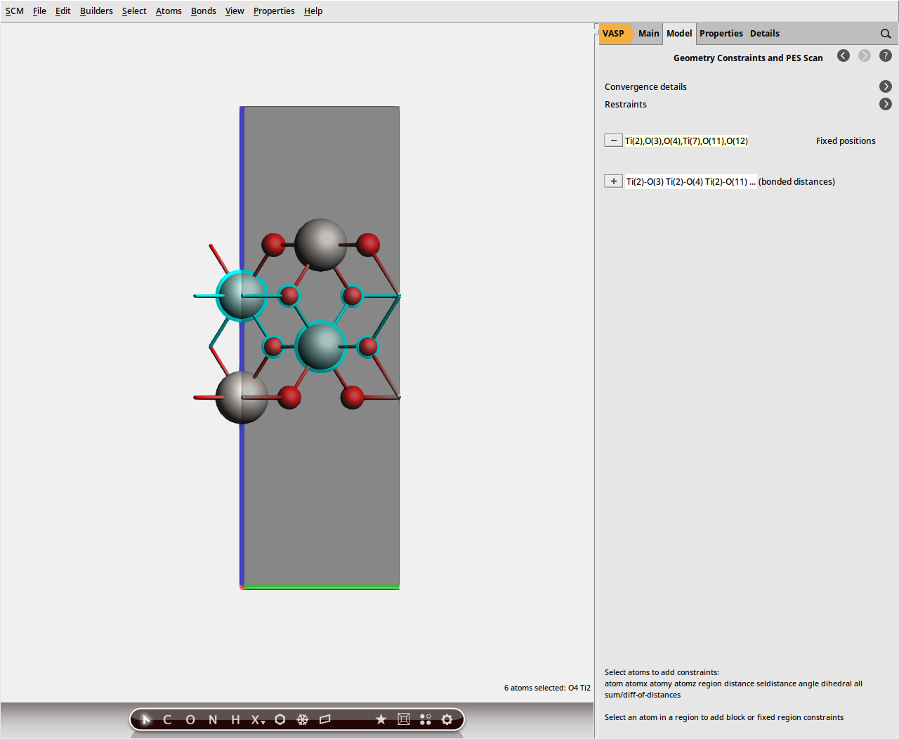
7. In the menu bar, select File → Save, and save your job with the name VASP_PBE_U_TiO2_slab.ams.

Note

When running VASP via the AMS driver, the geometry optimization settings and constraints are set for the AMS driver and not for VASP. This means that the VASP geometry convergence criteria, such as EDIFFG, do not need to be provided. The Selective Dynamics option will also be handled automatically by AMS.

Step 6: Run the job

1. Open AMSjobs: SCM → Jobs.

2. Select your job in the list. In the menu bar, select Queue → Interactive if you want to run the job on your local machine, or select the queue for the remote machine that you want to run on.

3. In the menu bar, select Job → Run.

After the calculation has finished, visualize the geometry optimization in AMSmovie.

4. Select your job in AMSjobs, and open AMSmovie: SCM → Movie.

5. In the menu bar, select View → Molecule → Balls

6. Use the horizontal scrollbar at the bottom of the window to navigate the geometry optimization steps.

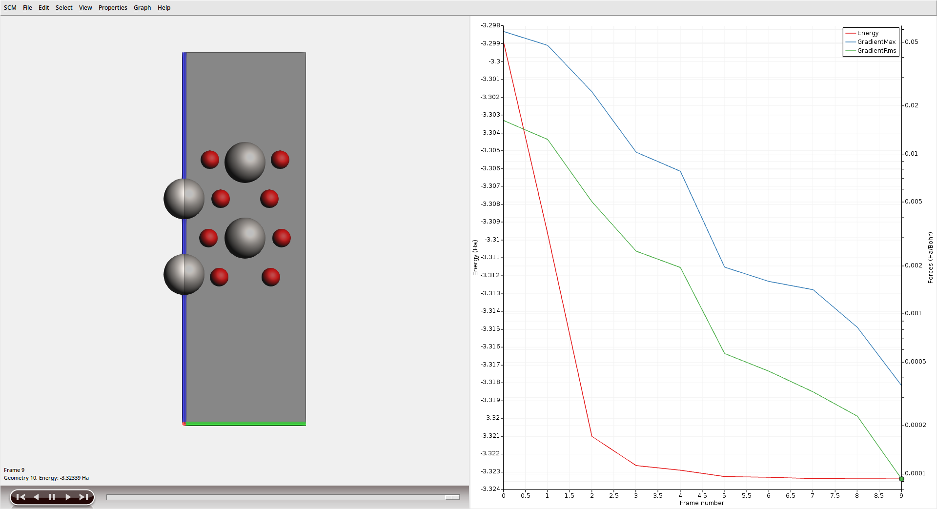
The Ti atoms in the outer layers can be seen to relax inwards towards the bulk as the optimization progresses.