Resonance Raman
In this tutorial we use the vertical gradient Franck-Condon (VG-FC) resonance Raman method
to calculate a resonance Raman spectrum in which the incident photon energy is close in energy to one of the excited singlet states of pyrene.
The VG-FC resonance Raman application needs all ground state vibrational frequencies and the electronically excited state gradient of the excited state of interest calculated at the ground state geometry.
More information on how resonance Raman is calculated in the VG-FC method can be found in the AMS user manual:
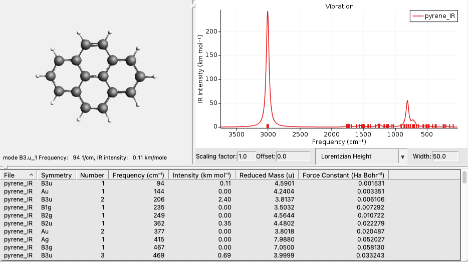
Let us first obtain a pyrene molecule. We optimize its geometry and calculate the vibrational frequencies with DFTB.
Start AMSjobs.
Click on SCM → New Input. This will open AMSinput.
In AMSinput, click the search icon

and type “pyrene” into the box.
Select the “Pyrene (ADF)” entry from the molecules section.
Click the Symmetrize button

to check the symmetry (should be D2h).
Select the DFTB panel:
 →
→ 
.
Check the Frequencies checkbox.
Select Model → DFTB3.
Select Parameter directory → DFTB.org/3ob-3-1.
Click on File → Save As… and give it the name “pyrene_IR”.
Click on File → Run.
Wait for the calculation to finish.
Click the ‘Update molecule’ button that pops up in the AMSinput window to update the geometry.
Click on SCM → Spectra.
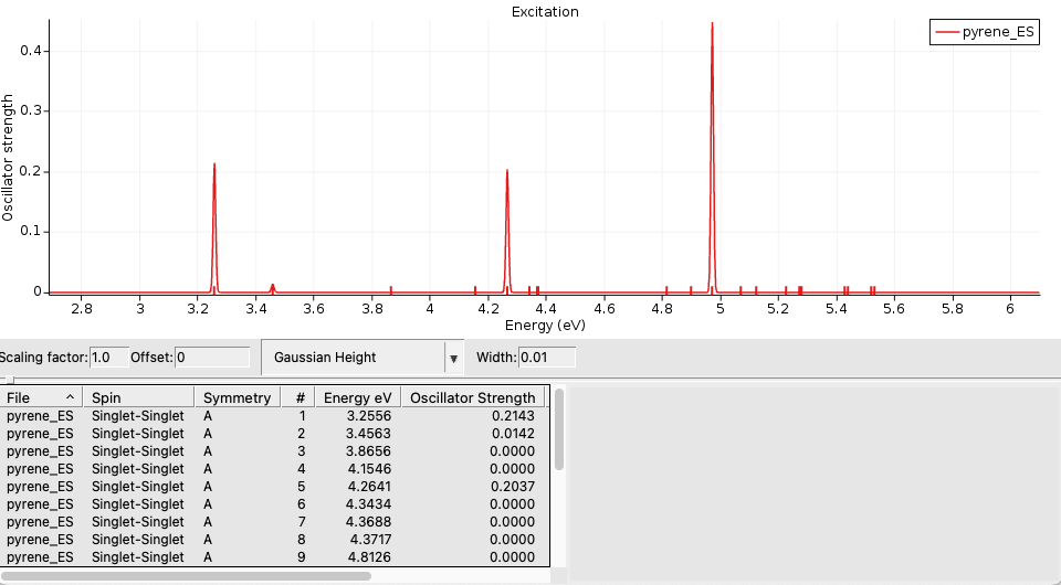
We calculate the excited state gradient of the lowest 11 excited states at the ground state geometry. This should give us multiple dipole-allowed excitations, allowing us to analyze different resonance modes.
Click on SCM → New Input.
Click on File → Import Coordinates (System) → From Files(s) and and select the “pyrene_IR.results/dftb.rkf” file.
Select the DFTB panel:
→ .
Select Task → Single Point.
Select Model → DFTB3.
Select Parameter directory → DFTB.org/3ob-3-1.
Panel bar Properties → Gradients, Stress Tenor.
Check the Nuclear gradients checkbox.
Panel bar Properties → Excitations (UV/Vis).
Select Type of excitations → Singlet.
Enter ‘20’ for Number of excitations.
Enter ‘1 2 3 4 5 6 7 8 9 10 11’ for Calculate excited state gradients for Excitation number.
Click on File → Save As… and give it the name “pyrene_ES”
(in the directory in which pyrene_IR.ams was saved).
Click on File → Run.
Wait for the calculation to finish.
Click on SCM → Spectra.
Axes → Horizontal Unit → eV.
Width → 0.01.
Axes → Horizontal Unit → cm-1.
The dipole allowed excitations are number 1, 2, 5, and 11.
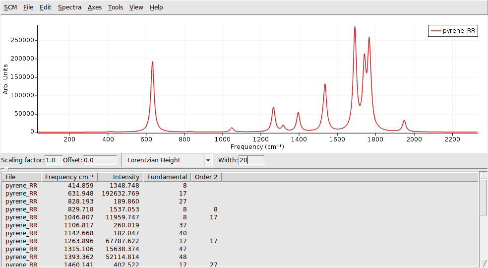
First we calculate a resonance Raman spectrum in which the incident photon is close in energy to the calculated lowest excited state at around 26000 cm-1.
For the VG-FC resonance Raman method we need a new input:
Click on SCM → New Input.
Click on File → Import Coordinates (System) → From Files(s) and and select the “pyrene_ES.ams” file.
Select the DFTB panel:
→ .
Select Task → Vibrational Analysis.
Select Model → DFTB3.
Select Parameter directory → DFTB.org/3ob-3-1.
Panel bar Model → Vibrational Analysis.
Select Type → Resonance Raman.
Click on the folder next to Mode file: and select pyrene_IR.results/dftb.rkf.
Check the All modes checkbox.
Click on the

next to
Excitation Settings.
Click on the folder next to Excitation file and select pyrene_ES.results/dftb.rkf.
Enter ‘A 1 2 5 11’ for Singlet.
Click on the

to go back to the previous page.
Click on the
next to
Spectrum Settings.
Enter ‘26000’ for Incident Frequency in cm-1.
Click on File → Save As… and give it the name “pyrene_RR”.
Click on File → Run.
Wait for the calculation to finish.
Click on SCM → Spectra.
Set the Width to 20 cm-1.
The peaks in the spectrum are at frequencies that correspond to fundamental vibrations (IR frequencies), combination bands (sum of different IR frequencies) and overtones (sum of identical IR frequencies). The default Raman order is 2, which means that the summation is over a maximum of 2 IR frequencies.
AMSspectra gives a list of frequencies and Raman intensities and the corresponding mode numbers of the IR frequencies involved. For fundamental frequencies only 1 mode number is shown. The mode numbers correspond to the numbers in an energy-ordered list of IR frequencies.
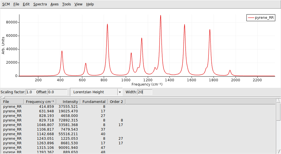
Next we calculate a resonance Raman spectrum in which the incident photon is close in energy to the calculated 11th excited state at around 40000 cm-1.
Click on SCM → Input (go back to the Input window).
Panel bar Details → Vibrational Analysis Spectrum.
Enter ‘40000’ for Incident Frequency in cm-1.
Click on File → Save As… and give it the name “pyrene_RR_11”.
Click on File → Run.
Wait for the calculation to finish.
Click on SCM → Spectra.
Set the Width to 20 cm-1.