Machine Learning Thermochemistry

MLPotential Thermochemistry

This tutorial will teach you how to:

• Download and install the ANI-1ccx machine learning (ML) potential parameter set [1] for organic molecules containing H, C, N, and O. ANI-1ccx was fitted to DLPNO-CCSD(T) reference data, which is a good approximation to CCSD(T).

• Calculate a gas phase reaction energy for an isomerization reaction using ANI-1ccx.

The above reaction is part of the ISOL benchmark set [2] for organic isomerization reactions. The CCSD(T)-calculated reaction (isomerization) energy is +5.30 kcal/mol. [3]

See also

• MLPotential documentation

• Thermochemistry with M3GNet

Installing ANI

When you set up a calculation with a ML model in AMSinput, the Graphical User Interface (GUI) will automatically prompt you to install it.

This installation is handled by AMSpackages. For ANI, you will see 2 package options: A CPU version and a CUDA version. Select the package that matches your system and install it when asked for.

Once ANI has been installed, it will also become available when running calculations through the Python library PLAMS.

Tip

You can also manually open AMSpackages to browse and install any of the other available ML models. AMSpackages is available through the main menu in the GUI: → Packages

Note

If you are using a remote queue to run AMS calculations, you will have to make sure ANI is installed on the remote system instead.

Set up and run ANI-1ccx calculations

You can set up and run the calculations for this tutorial using either the Graphical User Interface (GUI) or the python library PLAMS.

GUI

1. Start AMSinput.

2. Switch to ML Potential: →

3. Set the Task to Single Point.

4. Set the Model to ANI-1ccx.

5. Import the coordinates for Molecule 1 (see below), either using File → Import system or by copy-pasting the coordinates into the AMSinput window.

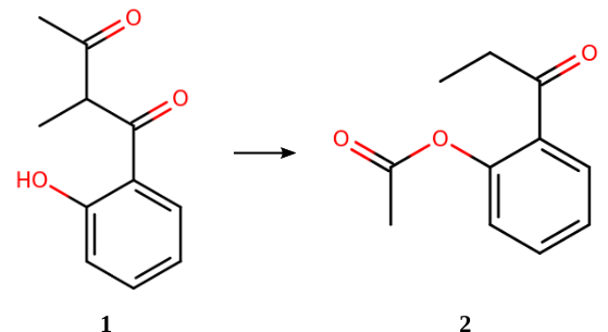
Molecule 1 (download e_14.xyz) [2]

26
IUPAC name: 1-(2-hydroxyphenyl)-2-methylbutane-1,3-dione, SMILES: CC(C(C)=O)C(=O)C1=CC=CC=C1O
C -3.24936 -0.212182 0.190882
C -3.01801 -0.0802601 1.55311
C -1.7187 0.143077 2.0465
C -0.658905 0.237377 1.15805
C -0.85036 0.110814 -0.240083
C -2.18086 -0.127187 -0.722042
C 0.257368 0.192893 -1.20091
O -2.46179 -0.277404 -2.02665
O 0.0637521 0.021523 -2.42106
C 1.687 0.513911 -0.736396
C 1.82965 1.96165 -0.236582
C 2.26431 -0.537731 0.241396
O 2.83801 -0.218511 1.26503
C 2.09562 -1.98435 -0.18481
H -4.2473 -0.390066 -0.201691
H -3.85485 -0.151744 2.24553
H -1.54519 0.241444 3.115
H 0.337705 0.411287 1.5486
H -1.5891 -0.204256 -2.50899
H 2.28669 0.397982 -1.65101
H 1.23053 2.14235 0.660044
H 1.50728 2.65825 -1.0195
H 2.87801 2.15978 0.0111843
H 2.38148 -2.11343 -1.23712
H 1.03194 -2.25389 -0.109562
H 2.68509 -2.64132 0.461071

6. Save the job with the name mol1singlepoint.ams.

7. If this is the first time you save a job with ANI-1ccx, AMSpackages will ask you to install the TorchANI backend. Choose between the CPU and CUDA versions and then select Install. It may take some time for the installation to complete. The installation requires a working internet connection.

8. Start the job: File → Run

9. Open the output file with AMSoutput: SCM → Output

Locate the energy in the section CALCULATION RESULTS:

CALCULATION RESULTS

Energy (hartree)          -651.36347065

Repeat the above steps for Molecule 2 (download p_14.xyz, or copy-paste the coordinates below)

26
IUPAC name: 2-propanoylphenyl acetate, SMILES: CCC(=O)C1=CC=CC=C1OC(C)=O
C -1.35638 2.12763 -0.654007
C -2.65222 1.75563 -0.292767
C -2.90548 0.454054 0.153058
C -1.86072 -0.467483 0.220499
C -0.53966 -0.111261 -0.111996
C -0.306066 1.21169 -0.548059
H -1.13871 3.125 -1.02877
H -3.46206 2.47839 -0.367275
H -3.9125 0.155448 0.435085
H -2.0661 -1.48038 0.55676
C 0.57311 -1.12022 -0.00101029
O 0.9385 1.6089 -1.01312
C 1.92817 2.11103 -0.153398
O 2.98828 2.39775 -0.635067
C 1.53429 2.27455 1.29711
O 1.68963 -0.797396 0.374748
C 0.239438 -2.56023 -0.391226
C 1.46196 -3.48021 -0.429606
H 0.619254 2.87262 1.3887
H 2.35794 2.7588 1.82629
H 1.34095 1.28633 1.72799
H -0.278681 -2.53555 -1.3614
H -0.505878 -2.93972 0.325436
H 2.19583 -3.11674 -1.15805
H 1.16125 -4.49774 -0.707814
H 1.95586 -3.51088 0.547894

The output for Molecule 2 should be

CALCULATION RESULTS

Energy (hartree)          -651.35251657

which gives a reaction energy of (-651.35251657) - (-651.36347065) = 0.010954 Hartree = +6.9 kcal/mol.

Python

Note

In order to use ANI with PLAMS, the ANI package has to be installed first using AMSpackages. See the installation instructions for more details.

1. Download e_14.xyz and p_14.xyz, which correspond to molecules 1 and 2, respectively.

2. Copy and save the script below with the name reaction.py.

3. Run the script using PLAMS: in a terminal, type $AMSBIN/amspython reaction.py. It will print the reaction energy.

4. Your calculation results are saved in the plams_workdir/ directory.

In the following python script (using the PLAMS library) we set up two single-point calculations using the MLPotential engine to determine the reaction energy.

import scm.plams as plams

s = plams.Settings()
s.input.ams.Task = "SinglePoint"
s.input.MLPotential.Model = "ANI-1ccx"

job1 = plams.AMSJob(name="mol1", settings=s, molecule=plams.Molecule("e_14.xyz"))
job2 = plams.AMSJob(name="mol2", settings=s, molecule=plams.Molecule("p_14.xyz"))

job1.run()
job2.run()

E1 = job1.results.get_energy(unit="kcal/mol")
E2 = job2.results.get_energy(unit="kcal/mol")
deltaE = E2 - E1

print("Energy molecule 1: {:.2f} kcal/mol".format(E1))
print("Energy molecule 2: {:.2f} kcal/mol".format(E2))
print("Reaction energy  : {:.2f} kcal/mol".format(deltaE))

Note

It can take a couple of seconds to initialize the ANI-1ccx model, which is quite long compared to the runtime of the calculation. If you want to run PLAMS calculations on multiple molecules using the same ML model, consider running them via the PLAMS AMSWorker:

import scm.plams as plams

s = plams.Settings()
s.input.MLPotential.Model = "ANI-1ccx"

molecules = {"molecule1": plams.Molecule("e_14.xyz"), "molecule2": plams.Molecule("p_14.xyz")}

with plams.AMSWorker(s) as worker:
    E = dict()

    for name, mol in molecules.items():
        results = worker.SinglePoint(name, mol)
        E[name] = results.get_energy(unit="kcal/mol")
        print("Energy of {} = {:.2f} kcal/mol".format(name, E[name]))

    print("Reaction energy: {:.2f} kcal/mol".format(E["molecule2"] - E["molecule1"]))

With a PLAMS AMSWorker, you can run calculations for many molecules while only performing the initialization once. This can save a lot of time for fast methods like ANI-1ccx.

Estimating reliability

Machine learning potentials give accurate predictions only for molecules or systems similar to those that were used during the parametrization of the machine learning potential. For other systems, the predictions may be very inaccurate.

The predictions (i.e. the energies) from the ANI potentials are averages over 8 separately trained neural networks (a neural network ensemble). The standard deviation of these individual predictions is used to estimate the reliability of the predicted values. If the predictions differ from one another (large standard deviation), then the molecule is probably not well represented in the training data.

The MLPotential output in AMS includes an “Energy uncertainty”. For example, for Molecule 1:

Engine energy uncertainty (hartree)              0.00212839

In this case, the standard deviation for Molecule 1 is 2.128 mHa = 1.3 kcal/mol. For Molecule 2, it is 1.8 kcal/mol. These uncertainties can be used when comparing energies with experimental data, or when performing sensitivity analyses on thermochemistry models. Some examples are provided in Refs. [1] and [4].

Note

The standard deviation grows with the square root of the number of atoms (assuming per-atom prediction errors follow a normal distribution). When comparing errors for molecules with a different number of atoms, it is therefore recommended to measure the standard deviation per root number of atoms.

Free energies, vibrational normal modes, and more

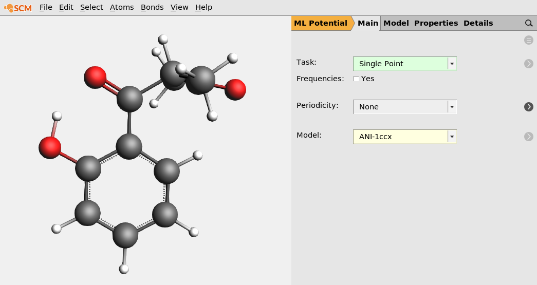
The molecular geometries provided in this tutorial have been optimized at a high level of theory. [2] You can also (re-)optimize them with ANI-1ccx:

1. Start AMSjobs.

2. Open the mol1singlepoint job with AMSinput.

3. Set the Task to Geometry Optimization.

4. Tick the Frequencies checkbox.

5. Save as mol1geo and run.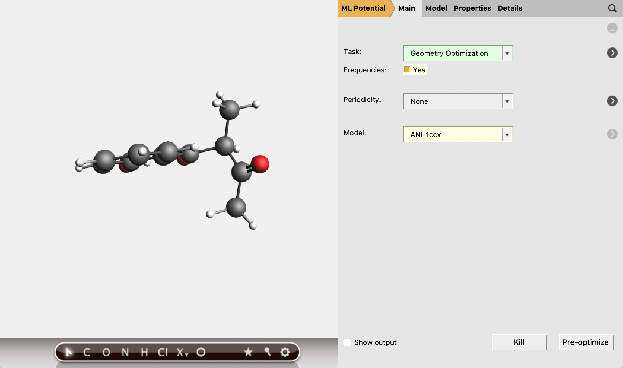

Look for Gibbs free energy in the output. (See also the Thermo keyword.)

1. Select the mol1geo job in AMSjobs.

2. Open it with the SCM → Output menu command.

3. In the search field at the bottom type ‘Gibbs’ to find the Gibbs free energy.

4. Visualize the normal modes in AMSspectra: SCM → Spectra.

Tip

ANI-1ccx geometry optimization jobs can be run interactively in AMSinput. Right-click on the pre-optimizer button , and select ANI-1ccx.

Note

The reaction energy above was calculated for particular conformations of the molecules 1 and 2. To explore all conformational isomers (conformers), see the Conformers tutorial.

Tip

If your organic molecules contain F, S, and/or Cl, you can run calculations using the ANI-2x model.

Tip

Consider using ANI-1ccx or ANI-2x to calculate a full approximate Hessian, and then use ADF to refine the vibrational modes that interest you.

Tip

By default, the ANI calculations will use all available CPU cores on your machine. To run a serial calculation, go to the Details → Technical panel and set Number of threads to 1.

On the same panel, you can also choose to run calculations on a CUDA-enabled GPU. See the parallelization section of the MLPotential manual for more details.

References

[1] (1,2)

J. S. Smith et al., Nat. Commun. 10 (2019) 2903. https://doi.org/10.1038/s41467-019-10827-4

[2] (1,2,3)

R. Huenerbein et al. Phys. Chem. Chem. Phys. 12 (2010) 6940-6948. https://doi.org/10.1039/C003951A

[3]

S. Luo, Y. Zhao, D.G. Truhlar. Phys. Chem. Chem. Phys. 13 (2011) 13683-13689. https://doi.org/10.1039/C1CP20834A

[4]

J. S. Smith et al., J. Chem. Phys. 148 (2018) 241733. https://doi.org/10.1063/1.5023802