Atomic Layer Etching of SiO₂

Semiconductors Atomic layer etching SiO2 ReaxFF Molecular dynamics Molecule gun

This tutorial will teach you how to:

• relax a silica slab with ReaxFF,

• define and configure an HF projectile, and

• run and inspect a molecule-gun molecular dynamics.

This tutorial is the GUI companion to AtomicLayerEtching.ipynb. The notebook builds the slab programmatically. In the workflow below, we use the prepared structure files so that the tutorial remains reproducible.

Introduction

Atomic layer etching (ALE) of SiO₂ using HF involves a self-limiting, two-step process to achieve precise, angstrom-level removal. It typically employs sequential exposure to hydrogen fluoride (HF) and a second reactant (like Trimethylaluminum) to modify the surface and remove the modified layer. In this tutorial, the first half-cycle is represented by HF molecules impinging on a hydroxylated SiO₂ slab.

The model uses three main ingredients:

• a hydroxylated SiO₂ slab,

• a frozen bottom region that anchors the slab and a thermostatted active region, and

• an HF molecule gun that inserts projectiles above the slab with a downward velocity.

The workflow consists of a ReaxFF geometry optimization followed by a ReaxFF molecular dynamics calculation with molecule insertion and removal.

Part A: Prepare the Hydroxylated Slab

The notebook constructs the SiO₂ slab from lattice vectors, cuts a surface, trims atoms at the top and bottom, and adds hydrogens to hydroxylate both exposed sides. Here we will start from the prepared XYZ file. You can also skip the relaxation and download the relaxed slab at the end of part C below.

Import the prepared slab

1. Open AMSinput: SCM → New Input

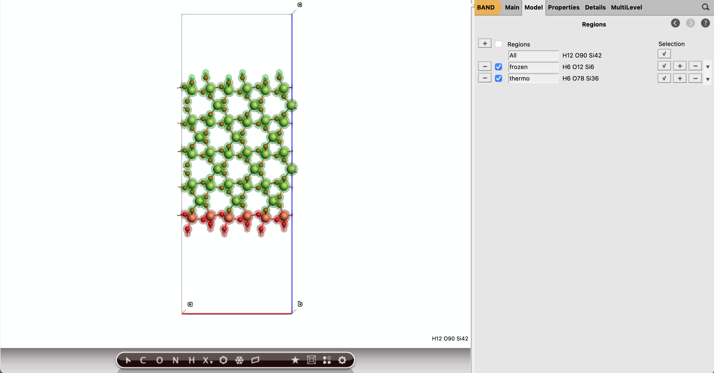
2. Import the prepared structure: File → Import Coordinates (System) and select SiO2_OH_slab_001.xyz

The molecular dynamics calculation treats the slab in two regions:

• frozen: atoms near the bottom of the slab, fixed during MD,

• thermo: all remaining slab atoms, controlled by a thermostat during MD.

Part A: Assign the regions

1. Rotate the slab to a side view (cmd/ctrl+2)

2. Select the atoms within about 3 Å of the bottom of the slab (at least include the first bottom layer of Si)

3. Create a new Region Model → Region and assign the selected atoms to a region named frozen

4. Select all remaining atoms (if you select the frozen region you can Select → Invert Selection)

5. Assign them to a region named thermo

6. Save the input as SiO2_slab_relax

Tip

The exact atom selection can be checked visually. The frozen region should form a thin support layer at the bottom of the slab, while the exposed upper surface should belong to thermo.

Part C: Relax the Slab

Before shooting HF projectiles at the surface, relax the hydroxylated slab with ReaxFF. This removes artificial strain introduced by slab construction and hydrogen placement.

Set up the ReaxFF geometry optimization

1. Switch to the ReaxFF engine: →

2. Set Force field to HONSiF.ff

3. Set Task to Geometry Optimization

4. Go to Details → GeometryOptimization

5. Set Optimize lattice to Yes

6. Save the job

7. Run the calculation

After the job finishes, open the optimized structure in AMSinput, update the molecule and save it for the MD calculation. The prepared relaxed structure is also available as SiO2_OH_slab_001_relaxed.xyz.

Part D: Create the HF Projectile

1. Start from the relaxed slab input

2. Press the F key, click above the slab to create a F atom, and press cmd/ctrl+E to passivate F and create HF

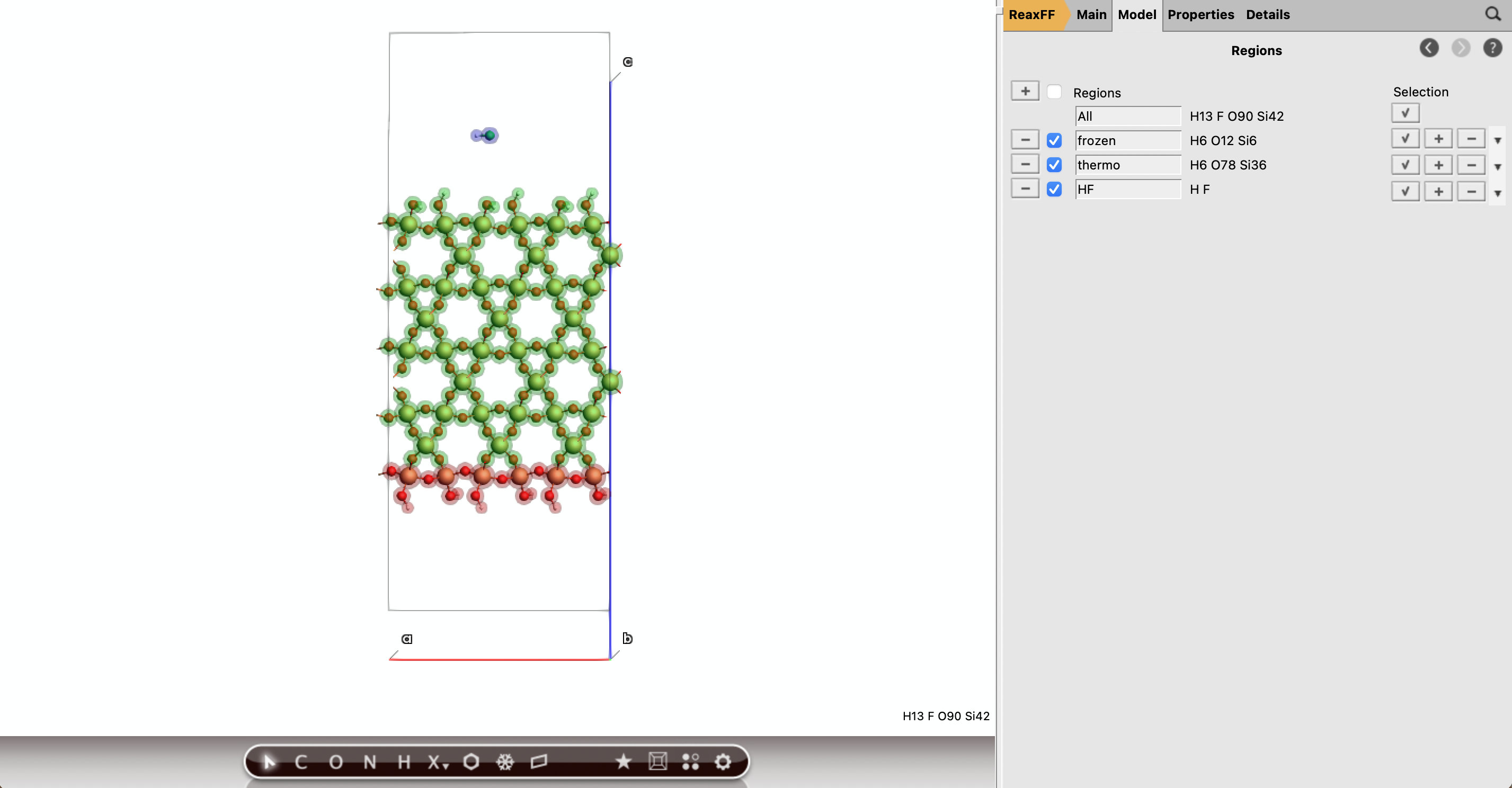
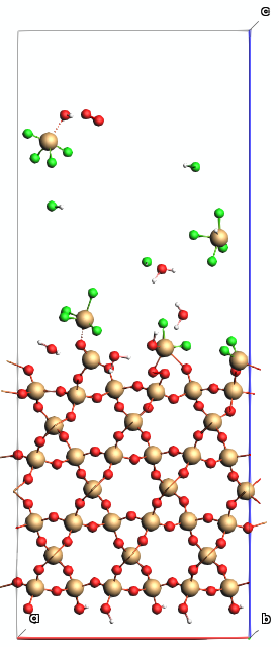
3. Model → Region, select the HF molecule and add a new HF region

4. Save the input

Part E: Configure Molecule-Gun MD

The half-cycle simulation inserts HF molecules above the slab and gives them a downward velocity. Molecules that leave the active region are removed with sink boxes.

Set the molecular dynamics task

1. From the Main panel set Task to Molecular Dynamics

2. Keep the ReaxFF engine and HONSiF.ff force field

3. Go to Model → MD

4. Set Number of steps to 100000

5. Set Initial velocities temperature to 100 K

6. Set the checkpoint frequency to a large value, for example 10000, to save 10 checkpoint files

7. Save the input

Configure the thermostat and constraints

1. Model → MD… → Thermostat and add a thermostat

2. Set the thermostat Type to NHC

3. Set Temperature to 300 K

4. Set Tau to 100 fs

5. Select the region thermo

6. From Model → Geometry Constraints and PES Scan select one atom from the frozen region and click the + to fixed the position of that region

7. Save the input

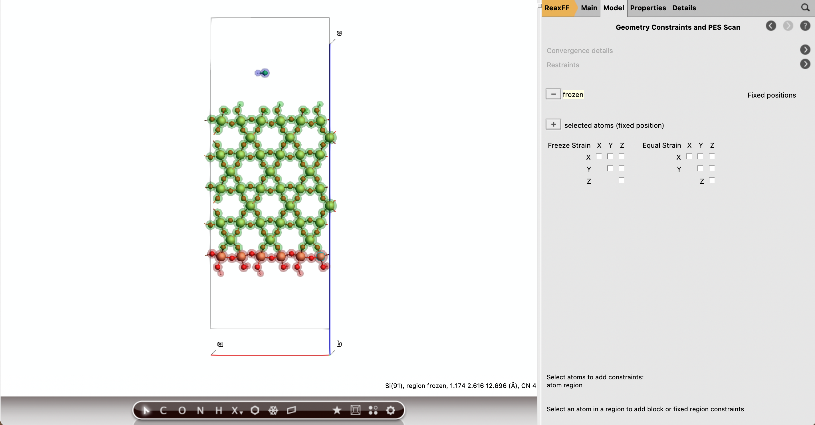
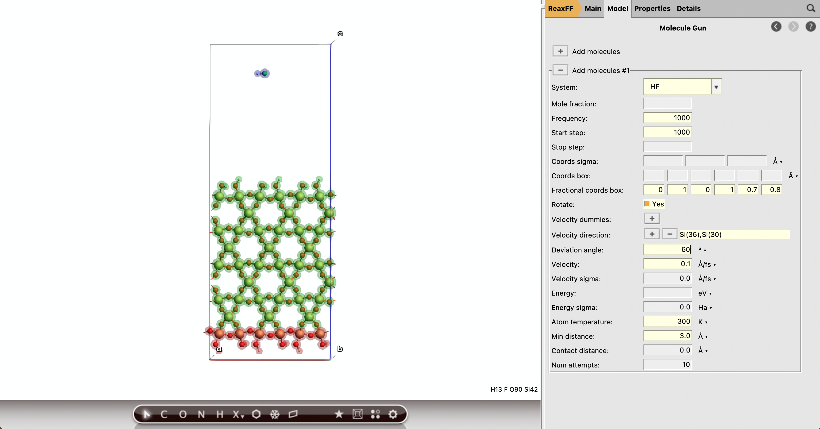
Add the HF molecule gun

Select the slab and move it such that the bottom of the slab is slightly above the z = 0 coordinates. Then you can Edit → Crystal → Map Atoms To (0..1) to have a clean setup.

1. Model → MD… → Molecule Gun, add an Add molecules block

2. Set System to HF

3. Set Frequency to 1000

4. Set Start step to 1000

5. Set Atom temperature to 300 K

6. Set Minimum distance to 3.0 Å

7. Set the insertion box to a thin slab above the surface, for example fractional coordinates 0 1 0 1 0.7 0.8

8. Select one Si atom hold the shift key, select another Si below and click the + to Set Velocity direction

9. Set Velocity to 0.1 Å/fs

10. Set Deviation angle to 60 degrees

11. Check the Rotate option and save

Tip

The insertion box should be placed above the relaxed surface, not inside the slab. In the notebook this position is computed from the top of the relaxed slab plus 6 Å.

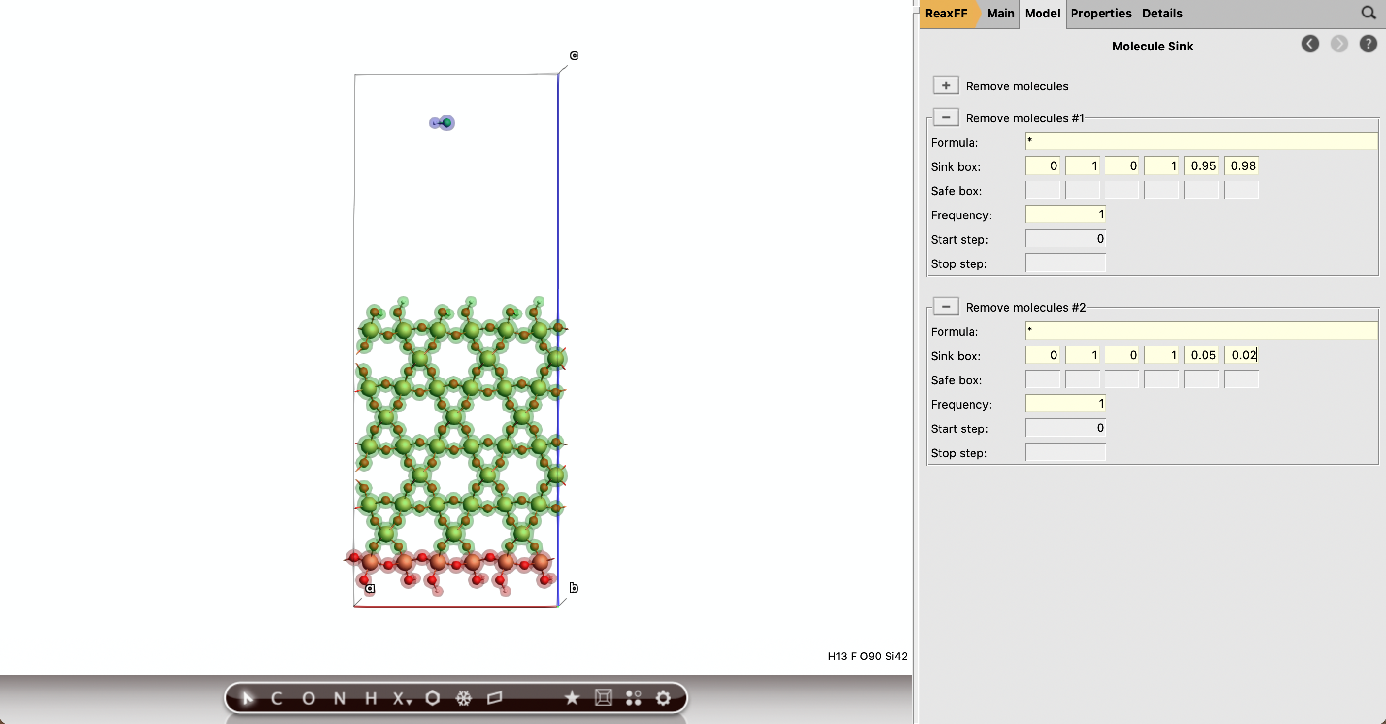
Add the removal sink boxes

1. Model → MD… → Molecule Sink Add a Remove molecules block

2. Set Formula to *

3. Set Frequency to 1

4. Add a Sink box with fractional coordinates 0.0 1.0 0.0 1.0 0.95 0.98

5. Add a second Remove molecules block

6. Set Formula to *

7. Set Frequency to 1

8. Add a Sink box with fractional coordinates 0.0 1.0 0.0 1.0 0.05 0.02

9. Save the job

Note

Be sure that the bottom of the slab is above the fractional coordinate 0.05 or the job might crash trying to remove an atom from a fixed region.

Run the calculation

1. Start the calculation with File → Run

2. Monitor the job in AMSmovie SCM → Movie

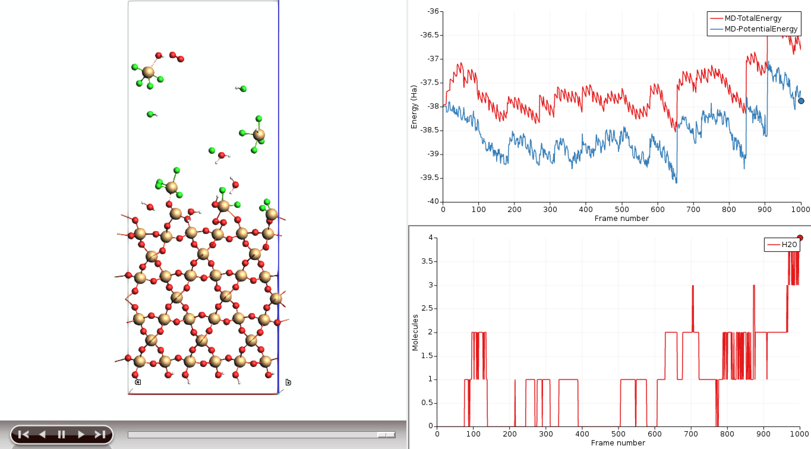
Part F: Inspect the Trajectory

After the MD calculation has produced trajectory frames, inspect representative structures in AMSmovie.

Analyze the molecule-gun trajectory

1. Open the results in AMSmovie

2. Play the trajectory from the beginning and confirm that HF molecules are inserted above the slab and that they are deleted reaching near the top of the supercell

3. Check that the projectiles move toward the surface

4. Inspect frames near impact events

5. Look for surface reactions, bond breaking, bond formation, or desorbing fragments

6. Use the graphing tools to inspect the total energy over time

7. Inspect the molecules created Graph → Add Graph and MD Properties → Molecules, select H2O

Note

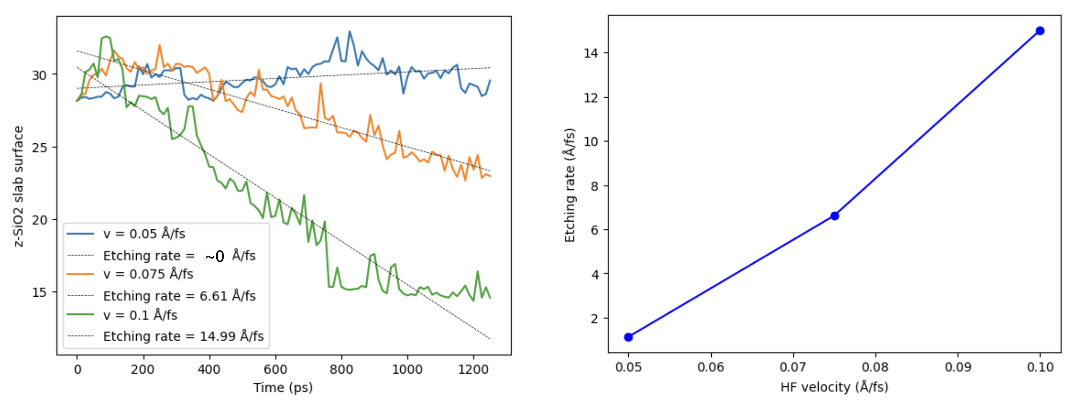
You usually want to run this simulation for many more steps to observe some important etching of the surface. The etching rates below were computed based on simulations of 1 ns.

Summary

The same setup can be adapted to other projectile molecules, slab sizes, impact velocities, and surface preparations. You can measure the top of the slab as a function of time and extract etching rates.