Quantum ESPRESSO: Magnetic Anisotropy Energy
In the pursuit of advanced spintronics and quantum computing, the miniaturization of magnetic units is a critical goal. However, a major challenge at the nanometer scale is thermal fluctuation, which can randomly flip the magnetic orientation of a device. The stability of a nanomagnet against these fluctuations is defined by its Magnetic Anisotropy Energy (MAE). MAE quantifies the energy barrier required to rotate the spin moment from a preferred stable direction (the “easy axis”) to a less favorable direction (the “hard axis”). For a storage device to function reliably, this energy barrier must be high enough to “block” thermal energy from flipping the bit. While many nanostructures (like nanowires or molecular magnets) exhibit MAEs of only a few meV (millielectronvolts), leading to low blocking temperatures (<50 K), practical applications require stability at room temperature. To frustrate thermal fluctuations at 300 K, the MAE must be unusually large, typically requiring values greater than 30–50 meV.
In this tutorial, we will focus on the Pt-Ir@SV-graphene system (a Platinum-Iridium dimer anchored on a Single Vacancy in graphene). This example is inspired on the paper:
Giant Magnetic Anisotropy of Transition-Metal Dimers on Defected Graphene by Jun Hu and Ruqian Wu Nano Lett. 14 (2014) 1853. In this paper, the authors investigated similar structures by changing the elements in the metal dimer. They investigated different 5d elements for the atom away from graphene (i.e., Os, Ir or Pt) and Fe group and Co group for the atom embedded in the carbon network (i.e., Fe, Ru, Os, Co, Rh, or Ir). They also considered Co−Co, Rh−Rh, and Ru−Ru dimers for comparison with the literature. Their research indicates that Pt-Ir@SV is the recommended candidate for robust nanomagnetic units. It possesses high structural stability and a giant positive MAE of 85 meV, well above the room-temperature threshold. The combination of giant MAE and the atomic scale of the dimer allows for incredibly high storage densities. For the system under consideration, the authors estimate a potential recording density of 190 TB/in² (Terabytes per square inch).
The goal of this tutorial is to learn how to set up the calculation and analyze the results to reproduce the high MAE of the Pt-Ir@SV-graphene system by using the Quantum ESPRESSO (QE) engine through the AMS driver.
MAE and the Force Theorem
The MAE is defined as the energy difference between two distinct spin orientations:
In this expression, the spin orientation is described by the spherical angles \(\theta\) and \(\phi\).
Why use the Force Theorem?
MAE can be calculated directly from self-consistent field (SCF) calculations that include Spin-Orbit Coupling (SOC). However, this is often computationally very expensive or simply prohibitive. Additionally, SOC calculations can be difficult to converge to the high level of precision required to resolve the tiny energy differences typical of MAE.
To address this, it is quite common to use the Magnetic Force Theorem. This theorem states that, to a leading order, the change in total energy due to a small perturbation (like a change in magnetization direction) can be approximated by the change in the sum of the single-particle Kohn-Sham eigenvalues. This bypasses the need for a full total energy recalculation.
Note
Please remember that the Magnetic Force Theorem is an approximation and should be used with caution, as it may not be valid for every physical system. However, a detailed discussion on the limits of its validity is beyond the scope of this tutorial.
The MAE is then evaluated as:
where \(\varepsilon_i\) represents the single-particle eigenvalues and \(f_i\) is the occupation number for state \(i\). The sum covers all occupied states. This approximation is highly accurate as long as the rotation of the magnetization does not significantly alter the self-consistent charge density or the potential.
Technical Workflow in AMS
From a technical point of view, the AMS driver internally orchestrates the required QE calculations, simplifying the workflow by wrapping multiple steps into a single execution. This automation eliminates the need for manual data handling, making the Force Theorem approach as straightforward to perform in AMS as a standard SCF calculation.
The process begins with a Collinear SCF Calculation, which is a standard DFT run performed without Spin-Orbit Coupling. In this stage, the magnetization is treated as a scalar quantity where the “Spin Up” direction establishes the reference quantization axis. By convention, this axis is aligned with the z-direction (\(\theta = 0^°\)) to generate the self-consistent ground-state charge density. This initial step provides the converged electronic distribution that serves as the foundation for the energy evaluation, effectively capturing the electronic structure of the system in its scalar-relativistic or non-relativistic limit.
Once the ground-state density is established, AMS proceeds to a Non-Self-Consistent (NSCF) Calculation with SOC. During this second phase, the spin-orbit term is included in the Hamiltonian as a perturbation while the charge density remains fixed at the values obtained in the first step. The spin quantization axis is then rotated to the specific (\(\theta, \phi\)) orientations of interest, and the Hamiltonian is diagonalized only once for each direction. This allows for the extraction of the single-particle eigenvalues (\(\varepsilon_i\)) necessary to solve the MAE equation, bypassing the need for expensive self-consistent iterations and reducing significantly the total computational effort.
Calculation Setup
You may either build and optimize the system geometry yourself by following the steps in the section System Geometry (Optional) or use the coordinates provided below to proceed. If you are using your own results, open the optimized structure in AMSview, select the molecule (by holding Shift and dragging the mouse), and copy it with Ctrl+C (or Cmd+C on Mac). Alternatively, you can copy the atomic coordinates provided below. In any case, simply paste the data using Ctrl+V (or Cmd+V on Mac) directly into the molecule-drawing area of a new AMSinput window.
19

 C -1.21467214  -2.09534449  -0.14151149
 C  0.00000000  -2.79009879  -0.18370579
 C -2.42195763  -0.00426468  -0.14151149
 C -1.28486654  -0.74181804   0.21001852
 C -3.62496512   2.09287459  -0.29698472
 C -2.41629643   1.39504939  -0.18370579
 C  1.21467214  -2.09534449  -0.14151149
 C  2.41831111  -2.78953661  -0.31975229
 C  1.28486654  -0.74181804   0.21001852
 C -1.20728550   2.09960917  -0.14151149
 C  0.00000000   1.48363608   0.21001852
 C  3.62496513  -2.09287459  -0.35062158
 C  4.83161914  -2.78953661  -0.31975229
 C  2.42195763  -0.00426468  -0.14151149
 C  3.62496513  -0.69955055  -0.31975229
 C  1.20728550   2.09960917  -0.14151149
 C  2.41629643   1.39504939  -0.18370579
Ir  0.00000000   0.00000000   1.40352258
Pt  0.00000000   0.00000000   3.78578874
VEC1   7.24993025 0.00000000  0.00000000
VEC2  -3.62496512 6.27862377  0.00000000
VEC3   0.00000000 0.00000000 15.00000000
Ground State Density Setup
The following figure highlights the main panel where parameters such as smearing, energy cutoffs, and pseudopotentials are defined. For this system, we use the LDA functional and Ultrasoft (US) pseudopotentials from the pslibrary. To proceed, simply reproduce the configuration shown in the image within your AMSinput window. Key technical settings include a 40.0 Ry wavefunction energy cutoff and a 7×7×1 Monkhorst-Pack K-point grid. Note that we initially set the Fully Relativistic option to No, as this selection only affects the initial Collinear SCF stage.
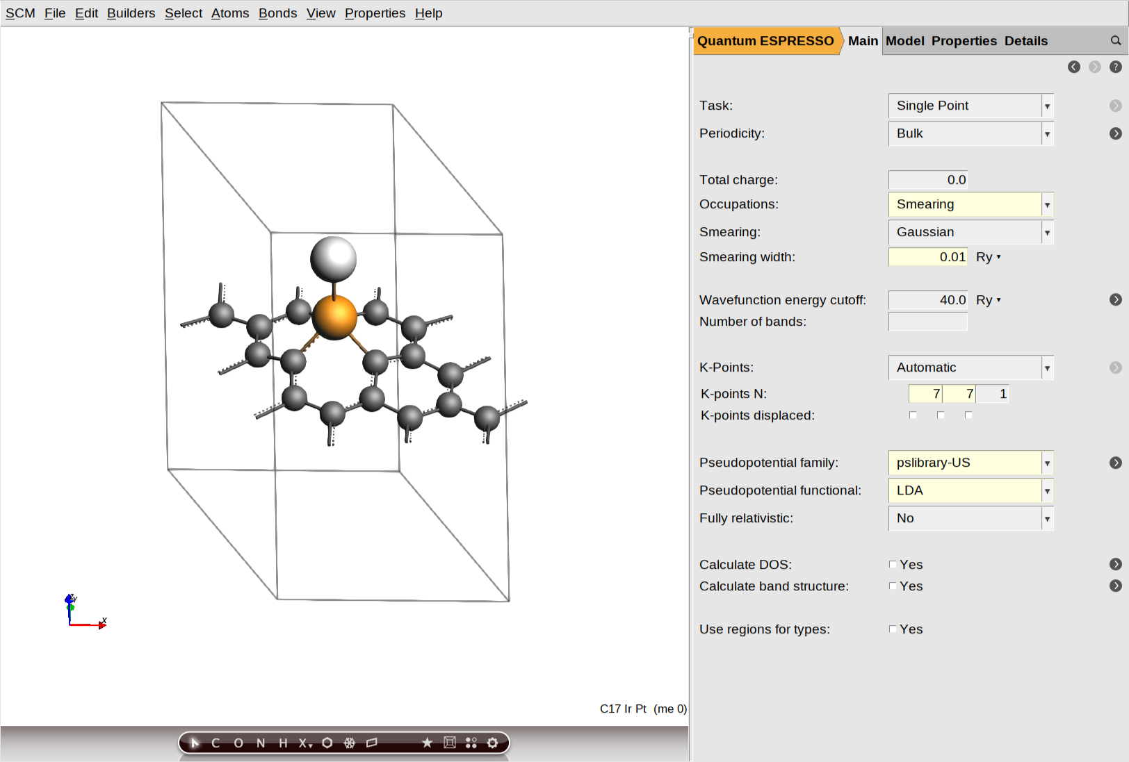
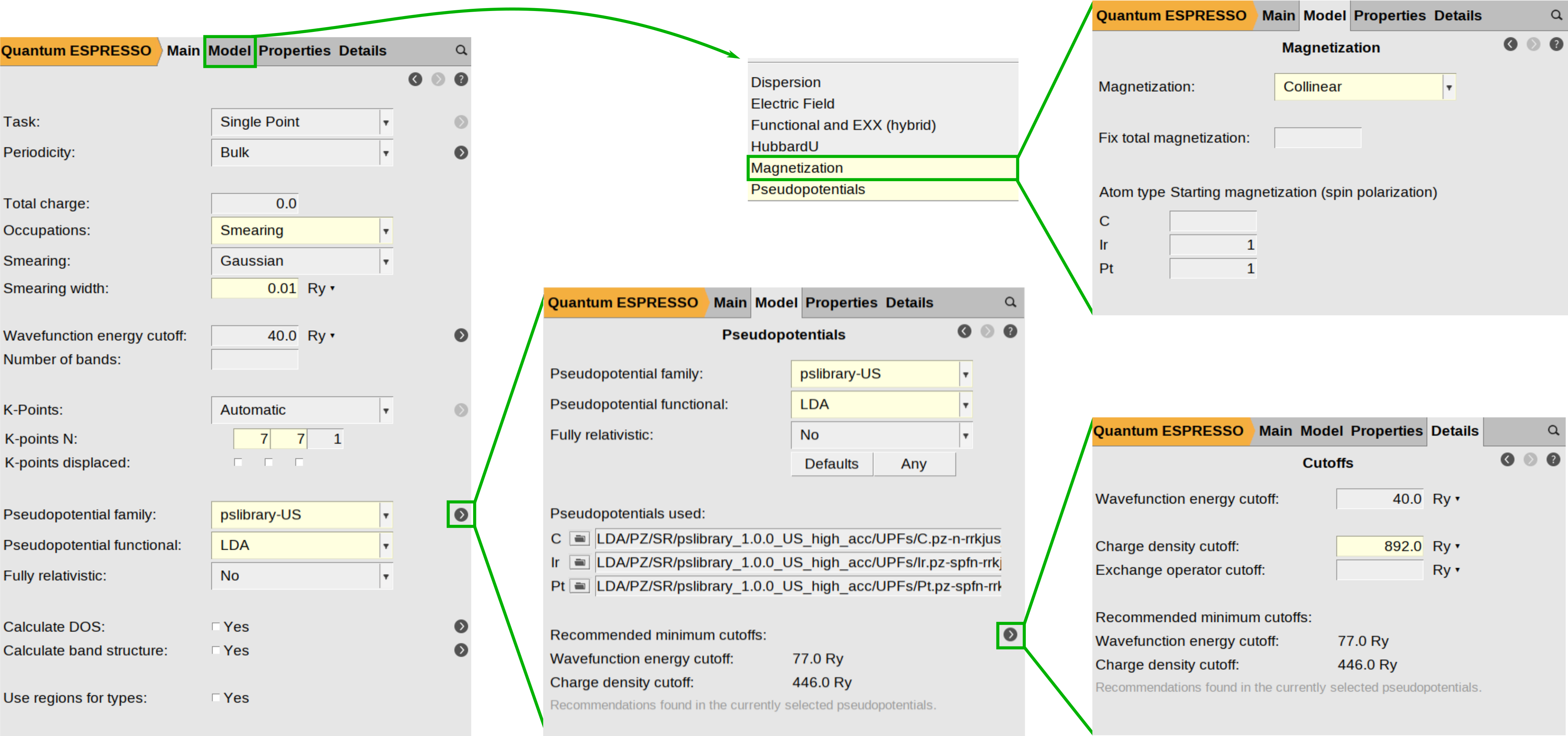
To begin setting up the magnetization parameters, navigate to Model → Magnetization and ensure the magnetization type is set to Collinear. In the atom-specific settings, define the initial spin polarization for Ir and Pt by entering 1 in the text box next to their atomic symbols.
While standard total energy calculations (such as structural relaxations) often treat the charge density cutoff (ecutrho) as a “set it and forget it” parameter linked directly to the energy cutoff (ecutwfc), typically ecutrho = 4*ecutwfc or ecutrho = 8*ecutwfc, calculating the MAE requires a much higher degree of precision. Because MAE relies on micro-electron volt (μeV) resolution, ecutrho becomes a critical, independent source of numerical noise that must be minimized. This parameter defines the resolution of the real-space FFT grid used to integrate the charge density and potentials. If the grid is too coarse, the atomic ions “feel” the discrete nature of the grid points.
As you rotate the magnetization (e.g., from Z to X), the shape of the electron cloud shifts slightly. If the grid is not fine enough to capture this subtle change smoothly, the resulting numerical noise can be of the same order of magnitude as the MAE itself (\(10^{−5}\) Ry). To ensure your results reflect physical anisotropy rather than grid noise, we recommend significantly increasing this value. In this example, we have manually adjusted the charge density cutoff to 892.0 Ry , twice the recommended value for this pseudopotential (446.0 Ry).
The following figure summarizes the steps described above:
Configuring Magnetic Anisotropy States
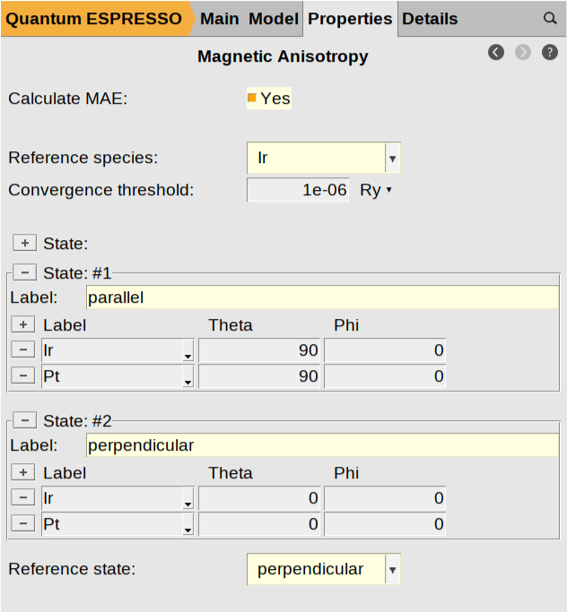
To complete the configuration of your magnetic states, from the AMSinput main panel, navigate to the Magnetic Anisotropy configuration panel by clicking Properties → Magnetic Anisotropy.
First, enable the calculation by checking the Calculate MAE: Yes box. Next, select Ir as the Reference species:, which sets the atomic type used as the primary axis for spin orientation. Add the specific magnetization directions you wish to compare by clicking the [+] button located to the left of State:. This allows you to include as many distinct states as you need. For this tutorial, add two states and label them parallel and perpendicular. Within each state, specify the spin orientation for both the Ir and the Pt atoms by entering the corresponding Theta (\(\theta\)) and Phi (\(\phi\)) angles. In this example, the parallel state is defined with a Theta of \(90^°\) (aligning the spins in the plane of the surface), while the perpendicular state uses a Theta of \(0^°\) (aligning them along the z-axis). Set Phi to \(0^°\) for all cases. Finally, use the Reference state text box at the bottom to select your baseline orientation. This selection defines the energy zero-point, allowing AMS to report the MAE of all other states relative to this reference, and in this case, we specify the perpendicular state.
Your configuration should look as follows:
Computation & Results
We are now ready to start the calculation
MAE_PtIr-SV-graphene)Once the calculation is complete, you can visualize and analyze your results using the AMSview module.
 plus sign, and select Magnetic Anisotropy
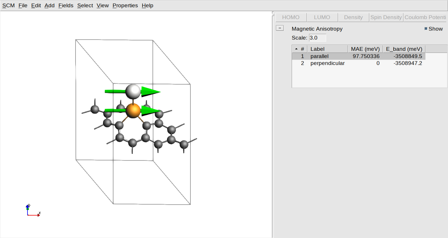
This tool provides a graphical representation of the magnetic properties and energy differences calculated in the previous steps.
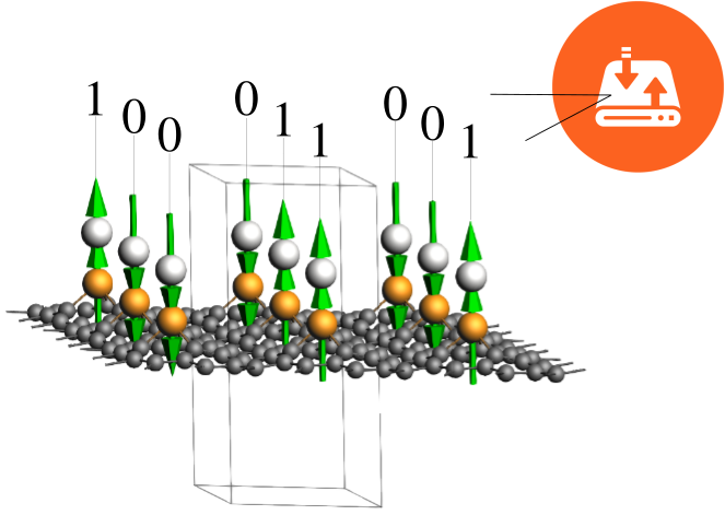
On the left-hand side, the molecular structure is shown with green vectors representing the magnetic moments for the specified atoms, allowing you to visually verify the spin orientations for each state. You can adjust the size of these vectors for better visibility by modifying the value in the “Scale:” text box. On the right-hand side, a results table provides the calculated MAE and Band Energy (E_band) values in meV. In this specific example, the MAE for the “parallel” state is approximately 98 meV relative to the perpendicular reference.
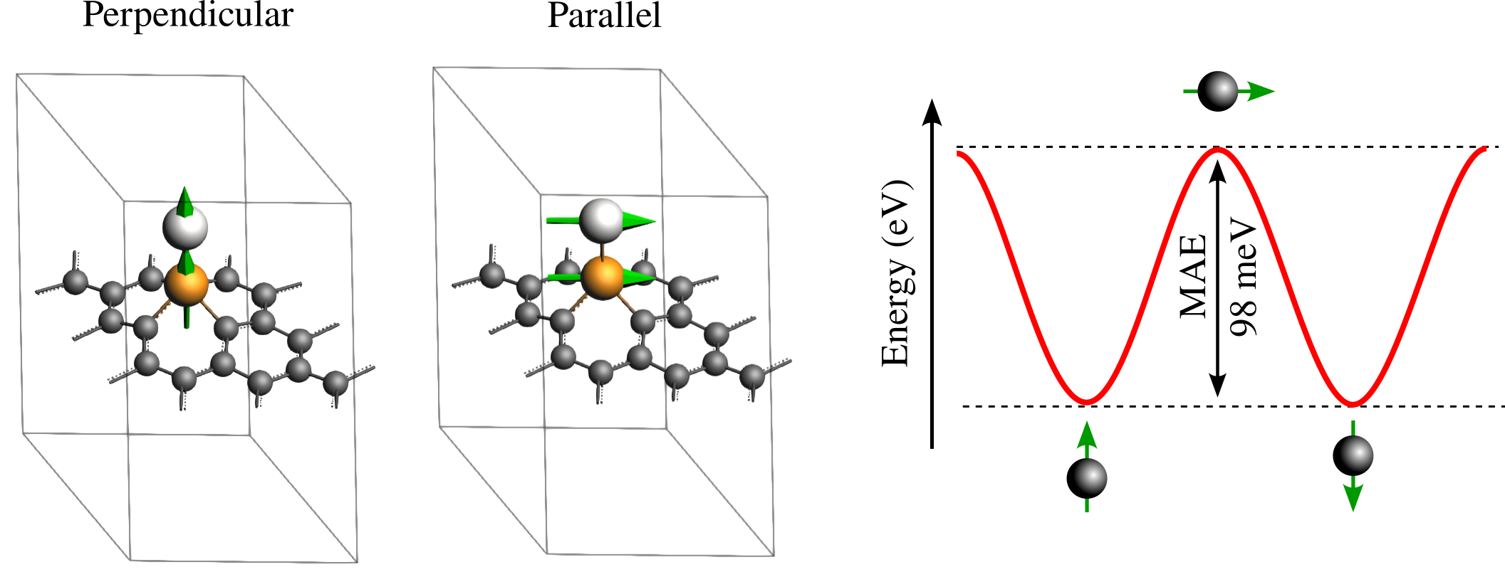
The figure above visually summarizes the results of the MAE calculation by correlating the atomistic magnetic configurations with their corresponding energy landscape. The left panel displays the atomic structures for the two calculated states: the stable “Perpendicular” orientation where magnetic moments align with the z-axis, and the higher-energy “Parallel” orientation where moments lie in the plane of the surface. The plot on the right illustrates the energy profile that would result from including intermediate angles between \(\theta=0^∘\) and \(\theta=180^∘\) by adding more states to the calculation. In this plot, the MAE is explicitly defined as the energy barrier, the difference between the maximum energy at the parallel state and the minimum energy at the perpendicular reference state. Note that the state at \(\theta=180^∘\) (moments pointing down) is symmetrically equivalent to the θ=0∘ reference and was therefore not explicitly calculated, though users are invited to verify this equivalence. While the resulting MAE of approximately 98 meV is a substantial value indicating high stability, it serves only as an initial estimate. To achieve the precision required to match literature references, a rigorous convergence study is necessary, which is out of the scope of this tutorial.
System Geometry (Optional)
We provide a simplified version how to create the molecular structure. For detailed guidance on structure manipulation and geometry optimization, please consult our dedicated tutorials.
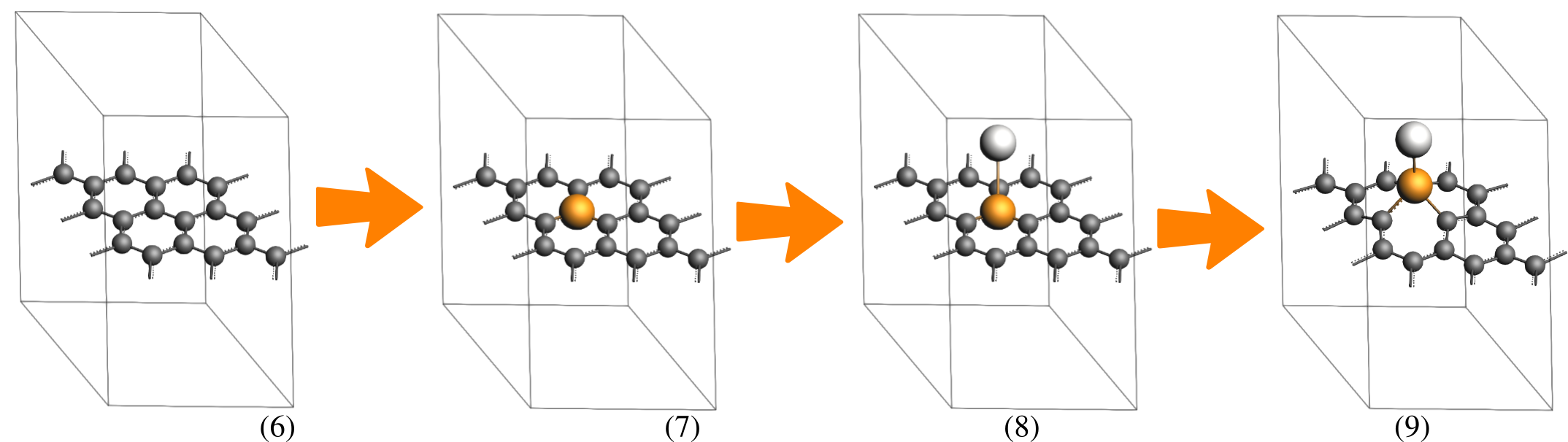
The numbered instructions below each figure describe the specific actions needed to achieve the geometry shown in that image.
We begin by creating a single layer of graphene 3x3. Starting from a predefined graphite structure, we will position a carbon atom at the center of the unit cell:
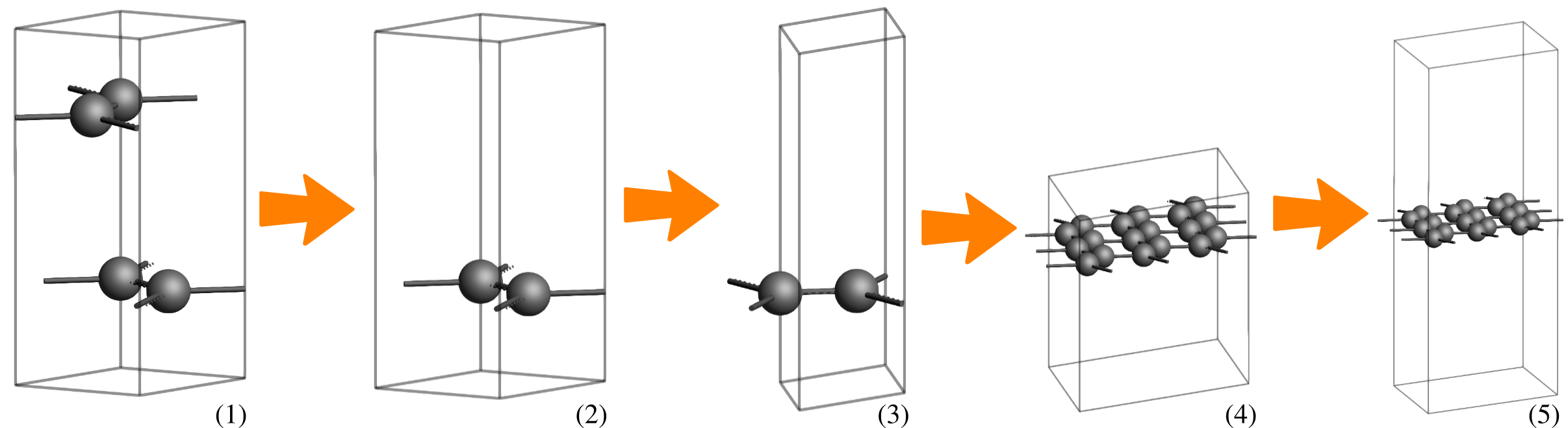
 search for
 Graphite and select Crystal → Graphite (Crystals-Hexagonal-Graphite). Optionally, change the following View settings:Delete.3, 3, 1 on the diagonal.15 angstrom Å, and then select Edit → Set origin … → Adjust Z only.Now, we optimize the graphene sheet using the QE engine with the LDA functional. Once converged, we replace the central carbon atom with an Ir-Pt dimer and perform a final geometry optimization also using the LDA functional to obtain our target system:
 →
→ 
 button to go to the optimization details. Check the Optimize lattice check box., and select Occupations:
 Smearing, Smearing width: 0.01 Ry, Pseudopotential family: pslibrary-US, and Pseudopotential functional: LDA. button on the side of the Task: GeometryOptimization option. Uncheck the Optimize lattice check box. Save and run the calculation.The final geometry optimization may take several hours.