Gibbs Free Energy in Heterogeneous Catalysis
The accurate calculation of Gibbs Free Energy (\(\Delta\text{G}\)) is a cornerstone in understanding the thermodynamics of heterogeneous catalysis and constructing reliable reaction energy diagrams. However, transitioning from gas-phase molecules to species adsorbed on a solid surface introduces significant complexity in treating vibrational, translational, and rotational degrees of freedom. In this tutorial, we show how to compute these properties using AMS, focusing on the prototype system of \(\text{CO}_2\) adsorbed on Pt(111). We will walk through three distinct methodological approaches: full phonon analysis using periodic boundary conditions, \(\Gamma\)-point vibrational analysis (also known as the Harmonic Approximation), and the Partial Hessian approximation, which restricts the frequency calculation to a reduced group of atoms, typically the adsorbate atoms. By evaluating these three routes, this tutorial aims to provide practical insights into leveraging AMS’s tools to balance computational cost with chemical accuracy when describing the stability of reaction intermediates.
Specifically, this tutorial will show you how to:
Perform a full Phonon analysis to capture the complete vibrational component of the slab-adsorbate system, providing the most rigorous description of lattice and molecular vibrations.
Execute a vibrational analysis (\(\Gamma\)-point) to estimate free energy corrections using a molecular-like approach, ideal for rapid screening of adsorption stabilities.
Use the Partial Hessian approximation by isolating the vibrations of the adsorbed \(\text{CO}_2\) from the Pt(111) surface, effectively reducing computational cost but sacrificing accuracy for the adsorbate’s thermochemistry.
Through these three steps, you will learn to create the corresponding AMS input files and how to extract the necessary thermodynamic data from the output files.
Performing these calculations manually for each state is instructive and sometimes necessary for complex cases requiring specific user oversight, but it can be tedious for routine screening. To address this, the last two sections of this tutorial illustrate how to use the PESExploration module to automate the process. We will show how to use this feature to compute the full Gibbs Free Energy profile in a single run.
System Description & Computational Details
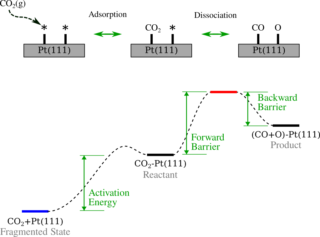
In this tutorial, we investigate the decomposition of \(\text{CO}_2\) on a Pt(111) surface. The reaction mechanism involves two steps:
Adsorption: \(\text{CO}_2\) from the gas phase adsorbs onto the Pt(111) surface. We refer to this adsorbed state as the reactant.
Dissociation: The adsorbed \(\text{CO}_2\) splits into adsorbed CO and O species. The final configuration is the product, and the process proceeds through a transition_state.
The figure below summarizes the process. The top panel illustrates the simplified mechanism: \(\text{CO}_2\) approaches the surface from the gas phase, adsorbs onto the Pt(111) slab, and subsequently dissociates into CO and O. The bottom panel maps these events onto a reaction energy profile, visually defining the key thermodynamic quantities we will calculate: the Activation Energy (the energetic cost to bring the molecule from the gas phase to the adsorbed reactant state), the Forward Barrier (energy required to reach the transition state from the reactant), and the Backward Barrier (energy required to reverse the reaction from the product).
Note
For simplicity, we assume the adsorption of \(\text{CO}_2\) (Gas \(\rightarrow\) Reactant) is a barrierless event. While detailed adsorption dynamics are crucial for kinetic modeling, they are outside the scope of this technical tutorial.
Here we chose the reactive force field (ReaxFF) engine in combination with the parameterization CHONSFPtClNi.ff, which has been specially designed to study the surface oxidation of Pt(111). In general, ReaxFF is highly efficient, allowing for rapid calculation of vibrational properties on large periodic systems.
Warning
We use ReaxFF here primarily for its speed to demonstrate the workflow. While ReaxFF is powerful, the reaction energies derived in this tutorial are illustrative and far from reality. For high-fidelity quantitative catalysis studies, one would typically employ electronic structure methods available in AMS through engines as e.g. BAND, Quantum Espresso, or DFTB. The procedure described here can be performed with any of these engines.
Setting up and running the calculations
In the figures below, you will find images of the molecular structures of the chemical systems we need, along with the corresponding files for download in XYZ format:
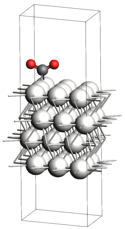
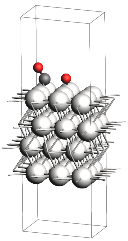
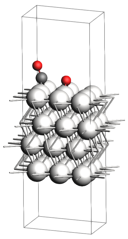

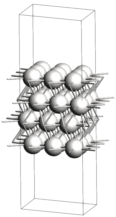
These structures are already optimized using the same Force Field. In particular, as expected, the transition state has one single imaginary vibrational frequency, corresponding to the reaction coordinate that connects the reactant and product (which can be verified by an IRC calculation). Technically, the reaction involves a \(\text{CO}_2\) molecule adsorbed at a top site which splits into a CO and an O atom, both adsorbing onto bridge positions.
Take a look at those xyz files. Notice that they have two non-standard attributes that are understood by AMS: regions and lattice vectors.
See below the last 9 lines of the file reactant.xyz.
Notice that the regions are specified at the end of each atom line, and the lattice vectors are specified at the end using the prefix VEC.
The region surface will be used to specify which atoms belong to the slab, while molecule specifies which atoms should be considered active in the Partial Hessian approximation.
Though not used in this tutorial, regions can also be used to specify constraints, such as fixing the bottom layers of the slab.
Pt       6.46873537       6.95546929       1.23929151   region=surface
Pt       6.46886538       2.15431307       1.24049406   region=surface
Pt       7.85480350       4.55449971       1.24126856   region=surface
C        5.08298061       2.18108236       9.94736863   region=molecule
O        5.08432103       3.32848735      10.50195851   region=molecule
O        5.08179422       1.03897381      10.51165774   region=molecule
VEC1       8.31557575       0.00000000       0.00000000
VEC2       4.15778787       7.20149984       0.00000000
VEC3       0.00000000       0.00000000      20.00000000
Notice that the \(\text{CO}_2\) file does not have a lattice. This is intentional. It is necessary to treat the gas-phase molecule as isolated to correctly account for its rotational and translational contributions to the entropy, which are absent in the adsorbed phase.
Now, you can download the complete example script from this link CO2-Pt111.run and execute it as shown below.
Do not forget to download the xyz files into the same directory.
$ bash CO2+Pt111.run
The script will run all necessary calculations. However, throughout this tutorial, we will walk you through its different sections. Please execute the command above now. These calculations should take about 10 minutes on a standard laptop. Most of the time is spent on the phonon calculations, the rest of the tasks take only a few minutes or even seconds.
OK, let’s start …
Full Phonon analysis
The most rigorous way to calculate the free energy of solid-state systems is via Phonon analysis. The Gibbs Free Energy (\(G\)) is defined as \(G = H - TS = U + PV - TS\). For solid-state systems at standard pressures, the \(PV\) term is negligible compared to the internal energy (\(U\)) and entropic terms (\(TS\)). Therefore, we can approximate the Gibbs Free Energy as the Helmholtz Free Energy (\(F\)):
The input file section below sets up the calculation. The meanings of its blocks are as follows:
System: Defines the geometry (imported from
reactant.xyz).Task GeometryOptimization: Ensures we are at a local minimum before calculating frequencies.
Properties Phonons Yes: Triggers the calculation of the phonons.
Engine ReaxFF: Configures the parameters of the engine.
20AMS_JOBNAME=reactant_phonons "$AMSBIN/ams" > reactant_phonons.out << EOF
21    Task GeometryOptimization
22    Properties Phonons=Yes
23    System
24        GeometryFile reactant.xyz
25    End
26    Engine ReaxFF
27        ForceField CHONSFPtClNi.ff
28    EndEngine
29EOF
The output file (reactant_phonons.out) contains several technical details, but most importantly, the thermodynamic properties derived from the phonon calculation.
Look for the table “Thermodynamic properties from phonons”.
Since we are interested in the reaction at 400 K, locate the row corresponding to Temperature(K) = 4.000000E+02.
The column Free Energy(Hartree) corresponds to the Helmholtz energy (\(F\)), which we use as our approximation for \(G\).
========================================
Thermodynamic properties from phonons
========================================
Zero-point Energy (hartree)            0.05760994
Zero-point Energy (eV)                 1.56764611

=============================================================================================
 Temperature(K) Internal energy(Hartree)   Entropy(kB) Free Energy(Hartree) Specific Heat(kB)

   0.000000E+00             5.760994E-02  0.000000E+00         5.760994E-02     0.000000E+00
   1.000000E+00             5.760994E-02  8.376922E-04         5.760994E-02      3.795979E-03
...
   3.990000E+02             1.647318E-01  1.904671E+02        -7.593468E-02      1.097737E+02
   4.000000E+02             1.650795E-01  1.907419E+02        -7.653829E-02      1.097921E+02
   4.010000E+02             1.654272E-01  1.910161E+02        -7.714277E-02      1.098104E+02
...
   9.990000E+02             3.781614E-01  2.933058E+02        -5.497552E-01      1.136389E+02
   1.000000E+03             3.785212E-01  2.934195E+02        -5.506842E-01      1.136415E+02
=============================================================================================
...
    =====================
    CALCULATION RESULTS
    =====================

Energy (hartree)            -7.83513196
...
The energy contribution from the phonons calculation in AMS (the “Free Energy” column in the table) does not include the total electronic energy of the system. It only includes vibrational corrections (ZPE and thermal).
To compare with results from other methods described below, we must calculate \(G_{total} = E_e + F_{phonons}\), where \(E_e\) is the electronic energy from the engine.
Its value can be obtained from the output file in the highlighted line that starts with Energy (hartree) after the CALCULATION RESULTS section.
In this tutorial, we will use eV as the preferred unit of energy. Be careful to convert the Free Energy correction from Hartree to eV. For this particular case:
This procedure (Optimization + Phonons) must be repeated for the transition_state, product, and surface.
You can do this by replacing the word reactant with transition_state, product, and surface, respectively, in the input file section shown above.
Check the downloaded script for the full implementation. Then, collect all values of \(E_e\) and \(G\), we will analyze them later.
Notice that this phonon calculation does not apply to the isolated \(\text{CO}_2\) molecule. Its free energy must be calculated using the molecular vibrational analysis (Ideal Gas Rigid Rotor Harmonic Oscillator) described in the next section.
\(\Gamma\)-point Vibrational Analysis
As you may have appreciated, calculating full phonons is computationally expensive. Running the provided script, the phonon calculations consumed more than 99% of the computational time. This cost often makes phonon analysis unaffordable for routine screening. Most engines calculate phonons using a finite difference approximation on a supercell, which scales poorly with system size. Therefore, a sufficient approximation is often to calculate vibrations only at the \(\Gamma\)-point (the center of the Brillouin zone).
In the input file, this is triggered by Properties NormalModes=Yes.
Crucially, we define the temperature of interest using Thermo Temperatures=400.0.
57AMS_JOBNAME=reactant "$AMSBIN/ams" > reactant.out << EOF
58    Task GeometryOptimization
59    Properties NormalModes=Yes
60    Thermo Temperatures=400.0
61    System
62        GeometryFile reactant.xyz
63    End
64    Engine ReaxFF
65        ForceField CHONSFPtClNi.ff
66    EndEngine
67EOF
In the output (reactant.out), look for the Statistical Thermal Analysis section.
AMS provides a breakdown of:
Entropy: The entropic contribution (\(S\)).
Internal Energy: Thermal corrections to the energy (\(U\)).
Gibbs free energy: The final target value (\(G\)).
============================
Statistical Thermal Analysis  *** ideal gas assumed  ***
============================
...
    Temp                                                 Transl   Rotat    Vibrat    Total
    ----                                                 ------   -----    ------    -----

    400.00   Entropy (cal/mol-K):                         0.000   0.000   371.654  371.654
             Nuclear Internal Energy (kcal/mol):          0.000   0.000   101.541  101.541
             Constant Volume Heat Capacity (cal/mol-K):   0.000   0.000   214.407  214.407
         (c) Constant Volume Heat Capacity (cal/mol-K):   0.000   0.000   185.131  185.131

    Summary of energy terms
                                          hartree           eV     kcal/mol       kJ/mol
                             --------------------  -----------   ----------  -----------
    Energy from Engine:        -7.835131964120705    -213.2048     -4916.62    -20571.14
    Nuclear Internal Energy:    0.161816248193982       4.4032       101.54       424.85
(c) Nuclear Internal Energy:    0.142120666965567       3.8673        89.18       373.14
    Internal Energy U:         -7.673315715926722    -208.8015     -4815.08    -20146.29
    pV/n = RT:                  0.000000000000000       0.0000         0.00         0.00
    Enthalpy H:                -7.673315715926722    -208.8015     -4815.08    -20146.29
    -T*S:                      -0.236907582306557      -6.4466      -148.66      -622.00
(c) -T*S:                      -0.219336266121665      -5.9684      -137.64      -575.87
    Gibbs free energy:         -7.910223298233278    -215.2481     -4963.74    -20768.29
Note that for the reactant (and the other periodic systems like the surface or product), AMS automatically detects the periodicity. Consequently, the Translational and Rotational contributions to the Entropy and Internal Energy are set to zero, as the slab cannot rotate or translate. The \(PV\) term is also zeroed out.
This procedure (Optimization + Vibrational Analysis) must be repeated for the transition_state, product, co2, and surface. Check the full script for details.
Unlike the Phonon analysis, here we also calculate the \(\text{CO}_2\) free energy using this method.
In contrast, for the isolated \(\text{CO}_2\) molecule (co2.out), these translational and rotational terms will are non-zero and contribute significantly to the gas-phase free energy.
Collect all values of \(G\) for later analysis. For the reactant case shown above: \(G = -215.2481 \,\text{eV}\)
\(\Gamma\)-point Vibrational Analysis & Partial Hessian Approximation
Calculating the Hessian for the entire surface slab is often unnecessary. The metal atoms in the bulk and surface are significantly heavier than the adsorbate, and their vibrations are often effectively decoupled from the reaction coordinate. The Partial Hessian Approximation drastically reduces computational cost by calculating second derivatives of the energy only for a selected subset of active atoms. In more complex cases, you can extend the active region to include specific surface atoms if their vibrations are strongly coupled to the adsorbate.
The input setup is nearly identical to the \(\Gamma\)-point analysis. We simply add a specification for the active region.
In our case, we defined molecule as the active region (SelectedRegionForHessian=molecule).
121AMS_JOBNAME=reactant_PH "$AMSBIN/ams" > reactant_PH.out << EOF
122    Task GeometryOptimization
123    Properties NormalModes=Yes SelectedRegionForHessian=molecule
124    Thermo Temperatures=400.0
125    System
126        GeometryFile reactant.xyz
127    End
128    Engine ReaxFF
129        ForceField CHONSFPtClNi.ff
130    EndEngine
131EOF
Below is the important section of the output file. Observe that the translational and rotational contributions are zero, as expected. Most notably, the vibrational contributions are much smaller than in the full analysis because we are ignoring the bulk lattice modes.
============================
Statistical Thermal Analysis  *** ideal gas assumed  ***
============================
...
    Temp                                                 Transl   Rotat    Vibrat    Total
    ----                                                 ------   -----    ------    -----

    400.00   Entropy (cal/mol-K):                         0.000   0.000    15.972   15.972
             Nuclear Internal Energy (kcal/mol):          0.000   0.000    15.810   15.810
             Constant Volume Heat Capacity (cal/mol-K):   0.000   0.000    11.224   11.224
         (c) Constant Volume Heat Capacity (cal/mol-K):   0.000   0.000     9.806    9.806

    Summary of energy terms
                                          hartree           eV     kcal/mol       kJ/mol
                             --------------------  -----------   ----------  -----------
    Energy from Engine:        -7.835131964120701    -213.2048     -4916.62    -20571.14
    Nuclear Internal Energy:    0.025195608038802       0.6856        15.81        66.15
(c) Nuclear Internal Energy:    0.024256233113602       0.6600        15.22        63.68
    Internal Energy U:         -7.809936356081900    -212.5192     -4900.81    -20504.99
    pV/n = RT:                  0.000000000000000       0.0000         0.00         0.00
    Enthalpy H:                -7.809936356081900    -212.5192     -4900.81    -20504.99
    -T*S:                      -0.010181400480265      -0.2771        -6.39       -26.73
(c) -T*S:                      -0.009126151883620      -0.2483        -5.73       -23.96
    Gibbs free energy:         -7.820117756562165    -212.7963     -4907.20    -20531.72
This procedure (Optimization + Vibrational Analysis with Partial Hessian) must be repeated for the transition_state and product. Check the full script for details, and collect all values of \(G\) for later analysis. For the reactant case: \(G = -212.7963 \,\text{eV}\).
For the \(\text{CO}_2\) molecule, we don’t need a new calculation. Since we treat the whole molecule, the partial Hessian is equivalent to the full Hessian.
Results
The table below summarizes the calculated Gibbs Free Energies and the resulting barrier heights for the three methods.
T = 400 K |
Gibbs Free Energy (eV) |
|||
|---|---|---|---|---|
Energy (eV) |
Phonons |
Full Hessian |
Partial Hessian |
|
Reactant |
-213.2049 |
-215.2482 |
-215.2482 |
-212.7963 |
Transition State |
-209.6474 |
-212.0116 |
-211.8783 |
-209.3745 |
Product |
-210.3997 |
-212.8065 |
-212.6857 |
-210.1851 |
\(\text{CO}_2\) |
-19.3909 |
-19.1666 |
-19.1666 |
-19.1666 |
surface |
-194.7569 |
-197.3883 |
-197.2092 |
-194.7569 |
Forward Barrier |
3.5575 |
3.2760 (0.0%) |
3.3699 (2.9%) |
3.4218 (4.4%) |
Backward Barrier |
0.7523 |
0.7949 (0.0%) |
0.8074 (1.6%) |
0.8106 (2.0%) |
Activation Energy |
0.9429 |
1.2673 (0.0%) |
1.1276 (11.0%) |
1.1272 (11.0%) |
There are two important points to clarify in this table: Firstly, notice that for the \(\text{CO}_2\) molecule, the Gibbs Free Energy is identical across all three columns. This is because phonons are not applicable to isolated molecules, and the Partial Hessian (when applied to the entire molecule) is mathematically equivalent to the Full Hessian. And secondly, for the surface in the Partial Hessian column, the Gibbs Free Energy (\(-194.7569\) eV) is identical to the raw electronic Energy. This occurs because the Partial Hessian approach ignores the vibrations of the surface atoms. Consequently, the surface is treated as a static environment with zero entropy and zero ZPE.
Regarding the accuracy of the methods, the table confirms that the Partial Hessian approximation introduces a larger error than the Full Hessian when compared to the benchmark Phonon calculations (4.4% vs 2.9% for the forward barrier). This is expected, as the Partial Hessian neglects the explicit coupling between the adsorbate and the surface lattice vibrations. However, more important are the physical insights revealed by the Gibbs Free Energy corrections. When we shift from raw electronic energy to free energy, the Activation Energy for adsorption increases significantly (from 0.94 eV to 1.27 eV), implying that the adsorption probability is lower than purely energetic models would suggest. In contrast, the Forward Barrier for dissociation decreases (from 3.56 eV to 3.28 eV), making the C-O bond breaking kinetically more likely, while the Backward Barrier increases slightly, making the recombination step more difficult.
Energy Landscape Refinement - \(\Gamma\)-point Vibrational Analysis
AMS offers a dedicated task called PESExploration which streamlines the calculation of reaction profiles.
Instead of running separate calculations for each state and manually collecting data, the Job LandscapeRefinement computes the entire profile in a single run.
The corresponding input file is shown below. The meanings of its blocks are as follows:
Systems: We define
System REACT,System PROD, andSystem TS. Note that the transition state definition links the reactant and product:System TS ts=yes reactant=REACT product=PROD.LandscapeRefinement: The keyword
GenerateFragments Yesautomatically identifies the adsorbate and surface fragments from the input geometries.StatesAlignment: We use
ReferenceRegion surfaceto tell AMS which atoms constitute the catalytic surface. TheDistanceDifference=0.5parameter is crucial here; since the surface atoms relax slightly differently in each state, this threshold (in Angstroms) allows AMS to correctly identify that the underlying surface is chemically identical across all states despite small geometric variations.Thermo Temperatures: As before, we set the temperature to 400.0 K.
161AMS_JOBNAME=landscape "$AMSBIN/ams" > landscape.out << EOF
162    Task PESExploration
163    Thermo Temperatures=400.0
164    PESExploration
165        Job LandscapeRefinement
166        LandscapeRefinement GenerateFragments=Yes
167        StatesAlignment ReferenceRegion=surface DistanceDifference=0.5
168    End
169    System REACT
170        GeometryFile reactant.xyz
171    End
172    System PROD
173        GeometryFile product.xyz
174    End
175    System TS ts=Yes reactant=REACT product=PROD
176        GeometryFile transition_state.xyz
177    End
178    Engine ReaxFF
179        ForceField CHONSFPtClNi.ff
180    EndEngine
181EOF
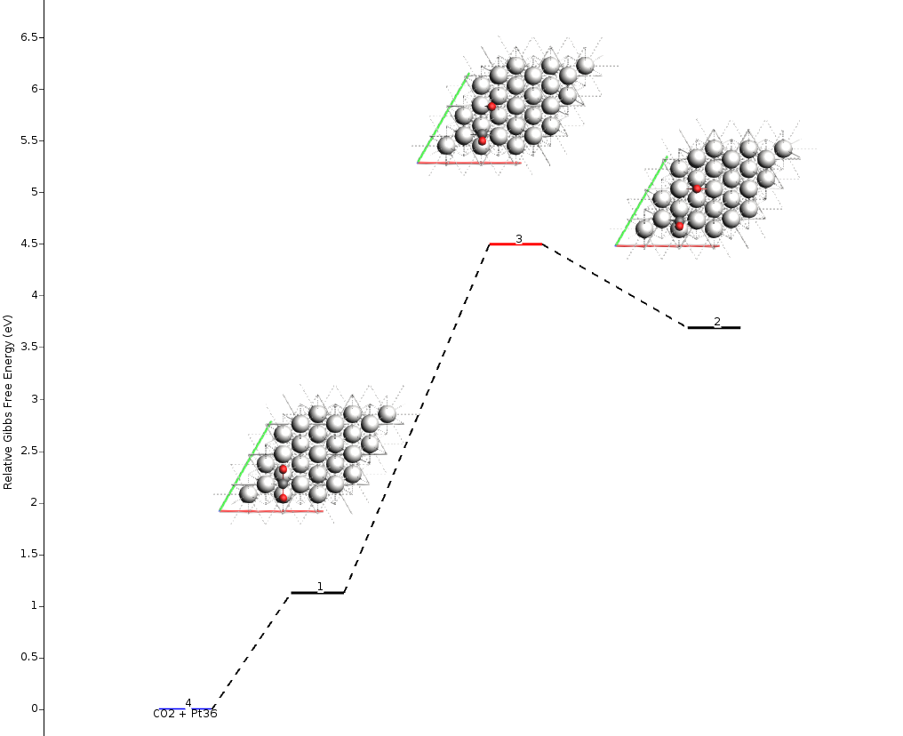
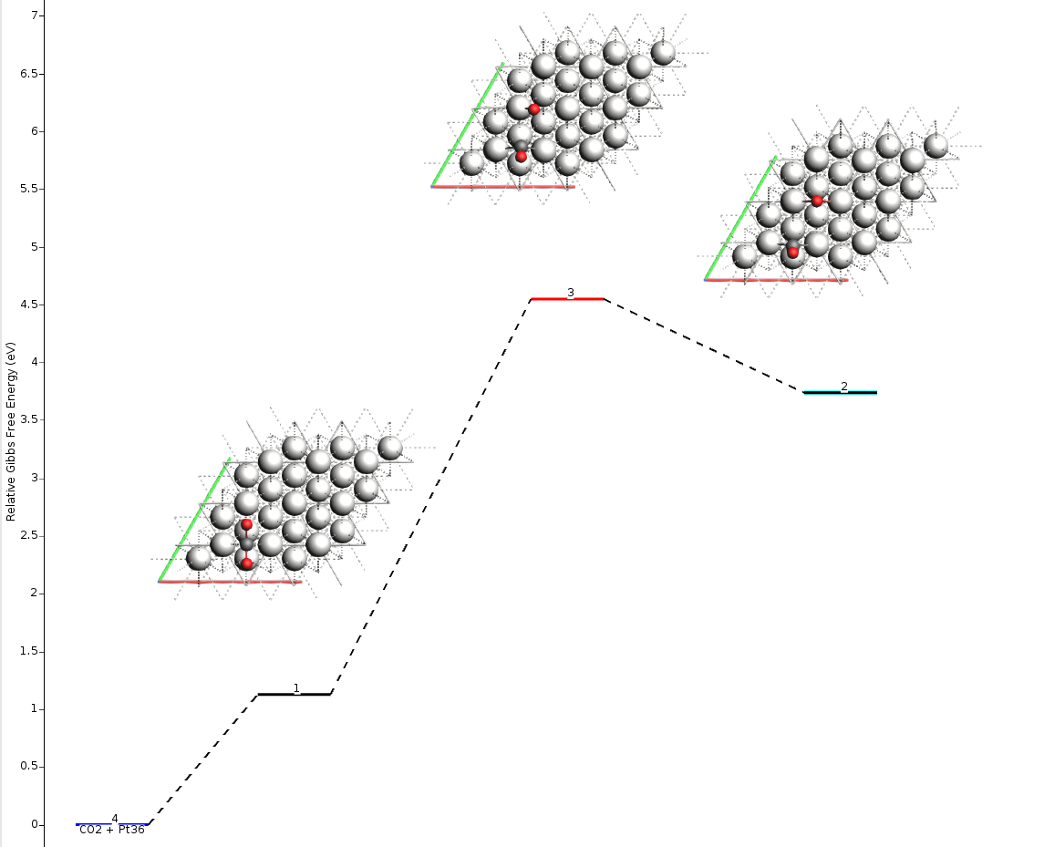
This single input generates the full Energy Landscape, which can be visualized using the AMSmovie command.
The barrier heights obtained here are identical to those calculated “molecule-by-molecule” in the previous sections.
$ amsmovie landscape.results
You should see something like this:
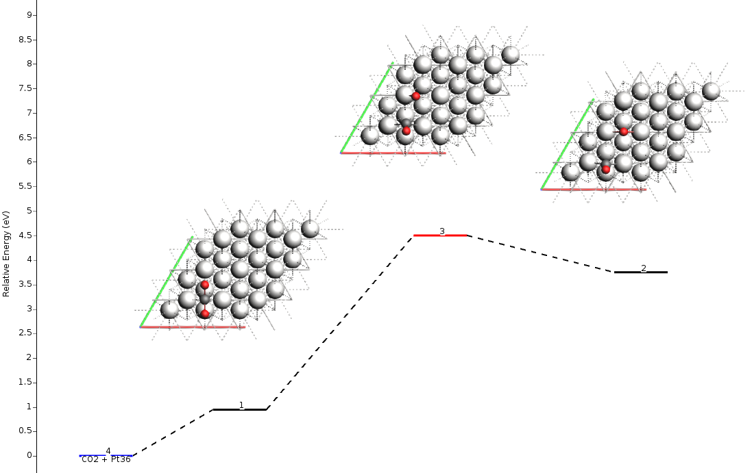
You can click on the states and move them to the left or right with Ctrl+Left arrow or Ctrl+Right arrow.
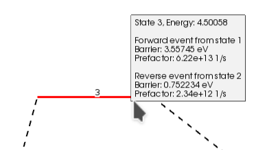
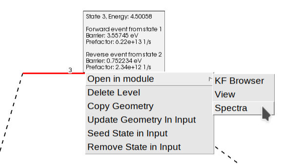
You can see the size of the barrier (Forward/Backward) by passing the mouse over the line that represents the transition state (red line). Notice that the values shown in AMSmovie are the same ones we found using the individual calculations in the table above:
From the AMSmovie menu bar, you can select Gibbs Free Energy:
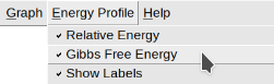
The reaction profile will update to show the Gibbs Free Energy:
In addition to seeing the energy barriers by passing the mouse over different states, you can right-click on top of it to open a context menu. This allows you to view the structure, the calculated properties (“Open in module” -> “View”), or inspect the vibrational spectrum (“Open in module” -> “Spectra”) to analyze vibrational modes and frequencies in detail.
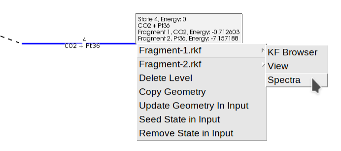
As we mentioned before, the option LandscapeRefinement GenerateFragments=Yes triggers the calculation of fragments.
One fragment represents the surface and the other represents the molecule. Their definition is based on the region surface.
The atoms outside of the region surface form the first fragment (\(\text{CO}_2\)), and the atoms inside that region form the second fragment (the surface).
The generation of fragments involves the geometry optimization of each fragment independently.
You can view the individual energies of the fragments by hovering over the fragmented state (blue line), or by right-clicking to access the “View” or “Spectra” options for a specific fragment (e.g., “Fragment-1.rkf” for the \(\text{CO}_2\)).
Energy Landscape Refinement - \(\Gamma\)-point Vibrational Analysis & Partial Hessian Approximation
Finally, we can combine the PESExploration workflow with the cost-saving Partial Hessian approximation.
The input is almost identical to the previous section, with one key addition: Properties SelectedRegionForHessian=molecule.
Here, molecule refers to the region defined for the \(\text{CO}_2\) adsorbate.
This tells AMS to calculate vibrational normal modes only for the adsorbate atoms, ignoring the surface modes.
The resulting energy landscape (shown below) is visually very similar to the full vibrational analysis, and the numerical values match exactly with the Partial Hessian results presented in the summary table above. This approach offers an optimal balance of precision and computational cost.
187AMS_JOBNAME=landscape_PH "$AMSBIN/ams" > landscape_PH.out << EOF
188    Task PESExploration
189    Properties SelectedRegionForHessian=molecule
190    Thermo Temperatures=400.0
191    PESExploration
192        Job LandscapeRefinement
193        LandscapeRefinement GenerateFragments=Yes
194        StatesAlignment ReferenceRegion=surface DistanceDifference=0.5
195    End
196    System REACT
197        GeometryFile reactant.xyz
198    End
199    System PROD
200        GeometryFile product.xyz
201    End
202    System TS ts=Yes reactant=REACT product=PROD
203        GeometryFile transition_state.xyz
204    End
205    Engine ReaxFF
206        ForceField CHONSFPtClNi.ff
207    EndEngine
208EOF
This is the result you would get for the energies:
$ amsmovie landscape_PH.results
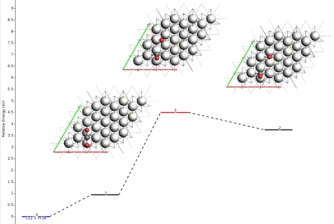
And this is the result in terms of Gibbs free energies:
Conclusions & Next Steps
In this tutorial, we have explored the calculation of Gibbs Free Energies for catalytic reactions on surfaces.
You have learned that while full Phonon calculations provide the highest accuracy by treating the complete lattice dynamics, they are often computationally prohibitive.
The Partial Hessian Approximation emerged as a powerful alternative, yielding relative barrier heights with errors of less than 5% compared to the full phonon treatment, but at a fraction of the time.
We also demonstrated how to automate this process using the PESExploration task, allowing you to generate comprehensive reaction energy profiles in a single run.
Armed with these thermodynamic data, a natural next step in your research might be to perform a microkinetic analysis to determine reaction rates and turnover frequencies under realistic operating conditions. You can explore AMS’s microkinetics MKMCXX or the pyZacros modules, to take your static energy landscapes into the realm of dynamic catalysis modeling.