Resin Blend from Molecular Dynamics

ReaxFF Molecular Dynamics Polymers Resin Miscibility RDF UFF Tomography

Resins are incorporated as a part of thermoplastic polymer formulations in order to alter the mechanical properties of the blend. This is used to improve extrusion or remolding compatibility through modified flow properties, or to tune viscoelastic characteristics of the product plastic during the hardening stage.

The miscibility of the resin is a key property affecting the structure of the polymer network. In this tutorial, we will showcase how to predict this network structure using molecular dynamics in AMS.

This tutorial will teach you how to:

• build a small polyisoprene/H-DCPD resin blend based on Ref. [1];

• monitor the blend density during thermal annealing;

• analyze the miscibility of the resin.

Introduction

Rissanou et al. [1] investigated hydrogenated dicyclopentadiene (H-DCPD) resin blended with polyisoprene (PI) and styrene-butadiene rubber (SBR). Resin miscibility was correlated to packing density, dynamic elastomer behaviour and stress responses.

This tutorial reproduces the outlined workflow, starting with the generation of the blend structure through simulated annealing. Packing inside the blend will be analysed using RDF and simulated tomography.

Note

You can also run this tutorial with Python using the companion notebook or the Python workflow.

For this tutorial, we provide the structures of the polymer and resin.

• PI_30mer.xyz

• HDCPD_trimer.xyz

Tip

Check out to the Building Polymers tutorial to learn how to build these polymer chain models yourself.

Create the Blend

The paper uses a system with a 10:23 molecular ratio of PI to H-DCPD. In order to determine the blend packing, we start with a structure consisting of 20 PI chains and 46 H-DCPD molecules. This produces a 10.000 atom system, which can run quickly on typical workstations.

1. Start AMSinput: SCM → New Input

2. Switch to the engine

3. Choose Builders → Packed Molecules

4. Set Density to 0.05 g/cm ³

5. Select Use number of molecules

6. In the first SMILES or file row, use the folder button to select PI_30mer.xyz

7. Set N mols for PI to 20 and Region to polymer

8. Click the to add a second row

9. In the second row, use the folder button to select HDCPD_trimer.xyz

10. Set N mols for H-DCPD to 46 and Region to resin

11. Click Generate molecules

12. Click Close to exit the builder

The builder has created a packing of rigid chains. To obtain a more realistic structure, we need to relax the molecules.

1. Set Task to Geometry Optimization

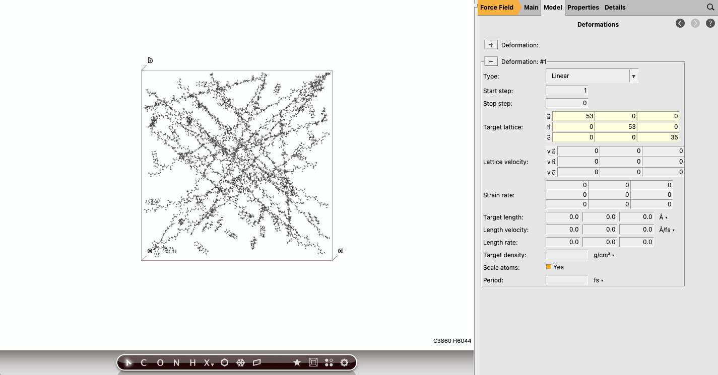
2. Save the job using File → Save as with the name UFF_InitialRelax

3. Perform the optimization using File → Run

This gives us a low-density structure. In order to obtain a structure with a density closer to the real material, we will compress the lattice. A rectangular unit cell will be used in order to improve contrast in the subsequent tomography analysis. We set up a molecular dynamics simulation to handle the relaxation of the dense structure:

1. Choose Update Molecule once the calculation is finished to load the optimized coordinates

2. Change the Task to Molecular Dynamics

3. In Model → MD, set Number of steps to 20000

4. Set Sampling frequency to 1000

5. Set Initial temperature to 5 K

6. Go to Model → MD… → Thermostat and add a new thermostat using the button

7. Set the Thermostat Type to Berendsen

8. Set the Temperature to 5 K

9. Set the Damping constant to 10 fs

10. Go to Model → MD… → Deformations add a new lattice deformation using the button

11. Set the target lattice with diagonal values 53 53 35 A

12. Save the job using File → Save as with the name UFF_Density

13. Start the simulation using File → Run

This calculation takes about 20 minutes on an Apple M2 with 16 GB of memory. After the simulation has finished, we can view the final density (around 1 g/mL) in the Properties → Properties (Including Estimated) menu.

Simulated Thermal Quenching

Experimentally, it has been shown that the properties of resin blends depend on the processing conditions. This is a result of the confined motion of the molecules in the blend. We will therefore simulate the quenching process after processing at elevated temperature in order to obtain a matching structure.

These simulations will be performed using the ReaxFF method in order to include bond (re)formation events during thermal processing. To start, we will re-optimize the UFF geometry of our high-density structure. This removes any artificial strain introduced by switching models:

1. Open the final structure from UFF_Density in AMSinput

2. Switch to the ReaxFF engine

3. Set Force field to dispersion/CHONSSi-lg.ff

4. Set Task to Geometry Optimization

5. Save the job using File → Save as with the name ReaxFF_InitialRelax

6. Perform the optimization using File → Run

Note

By using the cheaper UFF method for the initial optimization, we are able to shorten the duration of the ReaxFF optimization.

Having obtained a stable starting structure, we now set up a simulation for a thermal annealing cycle:

1. Open the final structure from ReaxFF_InitialRelax in AMSinput

2. Set Task to Molecular Dynamics

3. In Model → MD, set Number of steps to 25000

4. Set Sampling frequency to 500

5. Set Initial temperature to 413 K

6. Go to Model → MD… → Thermostat and add a new thermostat using the button

7. Set the Thermostat Type to Berendsen

8. To configure a heating/cooling cycle, change the Temperature field to 298.15 413 298.15 K

9. Set the Duration to 12500 12500

10. Set the Damping constant to 100 fs

11. Go to Model → MD… → Barostat and add a new barostat using the button

12. Set the Barostat Type to Berendsen

13. Set the Pressure to 1 atm

14. Set the Damping constant to 500 fs

15. Go to Model → MD… → Deformations add disable lattice deformations by using the button

16. Save the job using File → Save as with the name ReaxFF_Anneal_1

17. Start the simulation using File → Run

A single annealing cycle will likely be too short to stabilise the blend structure. We therefore repeat the annealing simulation several times:

1. Open the final structure from ReaxFF_Anneal_1 in AMSinput

2. Re-name the job using File → Save as to ReaxFF_Anneal_2

3. Start the simulation using File → Run

These cycles are repeated until the density stabilises to within 0.5 %. We can monitor this in AMSmovie:

1. Open AMSmoview with SCM → AMSmovie

2. Add a new viewport using Graph → Add Graph

3. Plot the density using MD Properties → Density

In total, 7 cycles were required in order to converge the system:

Table 12 Summary of the densities (in g/cm ³) obtained from the successive annealing procedures.

Annealing Step	Initial Density	Final Density	Last Third Average Density	% Change
1	0.8988	0.7290	0.7168	18.89
2	0.7290	0.7962	0.7917	9.22
3	0.7962	0.8377	0.8362	5.21
4	0.8377	0.8595	0.8580	2.60
5	0.8595	0.8744	0.8704	1.73
6	0.8744	0.8893	0.8871	1.70
7	0.8894	0.8932	0.8920	0.43

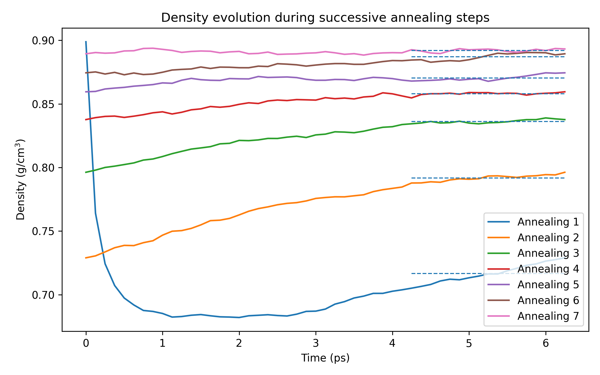
The final structure corresponds to the blend phase at 298.15 K.

A final MD simulation can be performed to determine the structural characteristics in the elevated temperature window at 413 K:

1. Open the final structure from ReaxFF_Anneal_7 in AMSinput

2. In Model → MD, set Number of steps to 50000

3. Set Sampling frequency to 100

4. Set Initial temperature to 413 K

5. Go to Model → MD… → Barostat add disable the barostat by using the button

6. Go to Model → MD… → Thermostat and change the Temperature field to 413 K

7. Save the job using File → Save as with the name ReaxFF_413

8. Start the simulation using File → Run

Comparison of these 2 structures allows us to see the effect of the resin both during the processing stage and in the final product.

Analyze the Trajectory

To understand the miscibility of the resin in the polymer matrix, we compute and report the resin-resin and resin-polymer center-of-mass radial distribution functions. You can use this PLAMS script to automatically handle the trajectory processing. We will focus on the 413 K phase here:

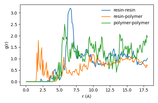
The resin molecules are seen to stick to the polymer chains, acting as structural spacers. This is also reflected in the decreased density of the blend compared to a pure polymer phase. [1]

A tomographic view of the miscibility can also be obtained by visualising the 2D density map of the resin molecules. A PLAMS script is provided to generate these images:

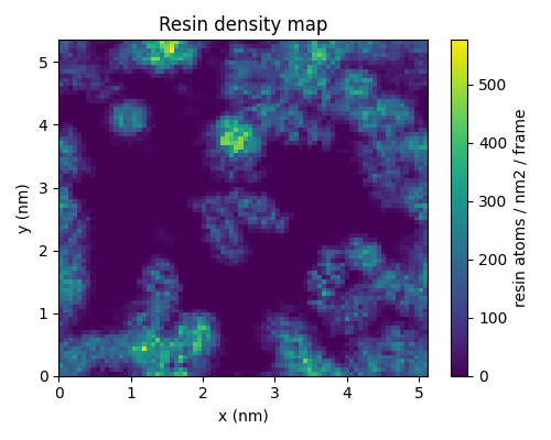
Alternating domains of polymer/resin material can indeed be seen. These images also highlight the formation of small resin-rich pockets inside the polymer matrix, accounting for the 4 Angstrom peak in the RDF.

Tip

To improve the resolution of the tomographic images, or lower the RDF noise, simulations can be performed for larger cell volumes to increase the amount of statistical data. Alternatively, longer MD simulations can be performed in order to increase the number of samples.

See also

Additional MD simulations can be used to characterise and compare the mechanical properties of the blend structures. See the following tutorials for more details:

• Glass transition temperature

• Stress/strain curves

• Thermal expansion coefficient

• Viscosity

References

[1] (1,2,3)

1. 14. Rissanou, R. Ghanta, M. Doxastakis, V. Harmandaris, Investigating the Role of Miscibility in Hydrogenated Dicyclopentadiene Resin/Polymer Blends: A Molecular Dynamics Study. Polymers, 18, 594 (2026)