Parameter Screening: Voltage Sweep
Simulation parameters can be screened in order to study device performance under different conditions, or to search for desired material properties. For this tutorial, we will perform a voltage sweep to predict the JV profile of an OLED device.
Note
A pre-made project file is available for this tutorial.
Create Materials
We start by creating the materials that are used in the stack.
NPD has a HOMO energy of -5.45 eV and a LUMO energy of -1.4 eV
mCBP has a HOMO energy of -6 eV and a LUMO energy of -1.5 eV
Ir(dmp)3 has a HOMO energy of -5 eV and a LUMO energy of -1.7 eV
For this tutorial, we will focus on charge transport only. The Transport template can be used when creating new materials. In the Electronic tab, we set the appropriate HOMO and LUMO levels. We will use a Gaussian DOS with a standard deviation of 0.1 eV for both polarons. Excitonic processes will be omitted for now.
Tip
Check out the Bulk Simulation tutorial for more details on adding new materials to a project.
Create Compositions
Navigate to the Compositions page to access the compositions that make up the device layers. Pure compositions for each of the compounds should already be available.
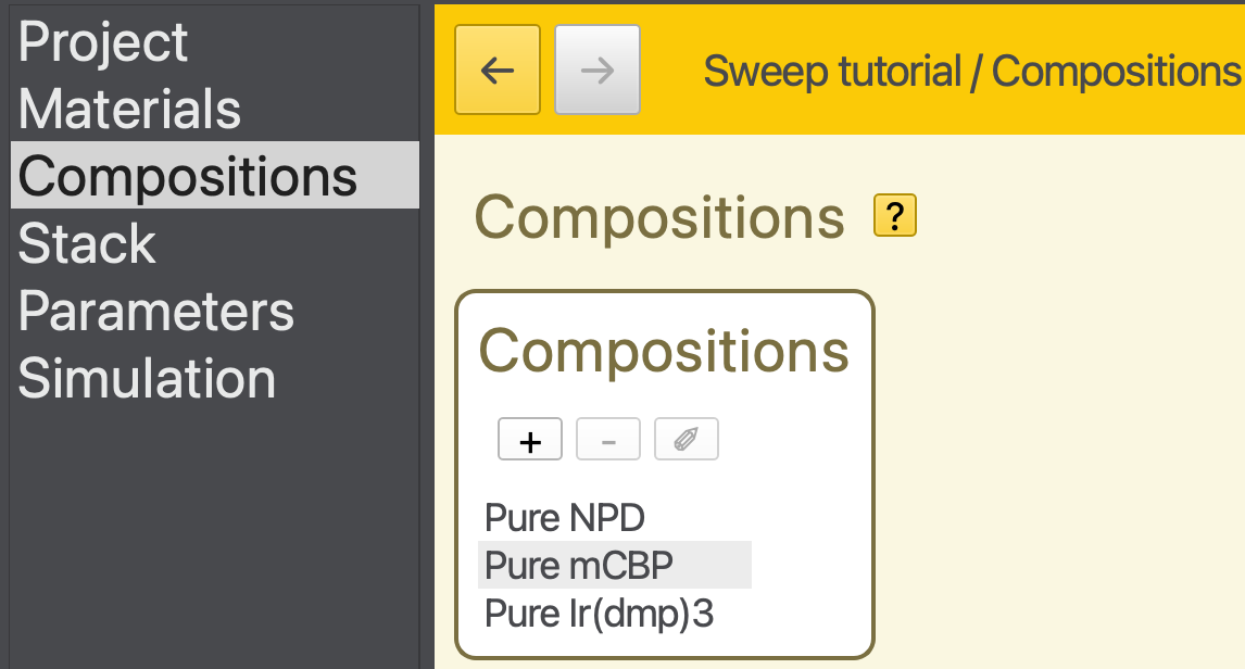
Fig. 24 Pure compositions have automatically been added to project
In addition, we are going to create a new host-guest mixture. Click on the  button in the table. This will bring you to the composition editor.
We will create a mixture of 0.9 mCBP and 0.1 Ir(dmp)3. To add a component to the mixture, simply click the in the Fractions table. A new material will be added to the composition. The mole fraction of a newly added material will, by default, be used to close the balance. (The first material will therefore always be given a fraction of 1.)
The Fractions table can be edited directly. We will adjust the materials and mole fractions in order to create the desired blend.
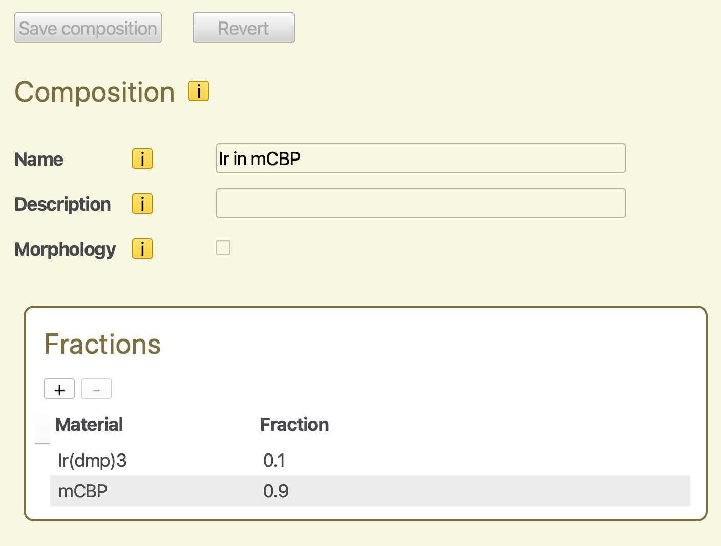
Fig. 25 Mixed composition for a host-guest system
Click the Save Composition button to add the host-guest mixture to the project. The Compositions page will now show four compositions in total.
Tip
You can also use the  to remove a material from the composition.
Create a Stack
We will create a stack using 3 layers. The outer contact layers are composed of pure NPD. The inner emitter layer contains the host-guest mixture defined earlier.
Create a 10 nm NPD layer
Create a 60 nm layer containing the mCBP-Ir(dmp)3 mixture
Create another 10 nm NPD layer
You will end up with an 80 nm stack.
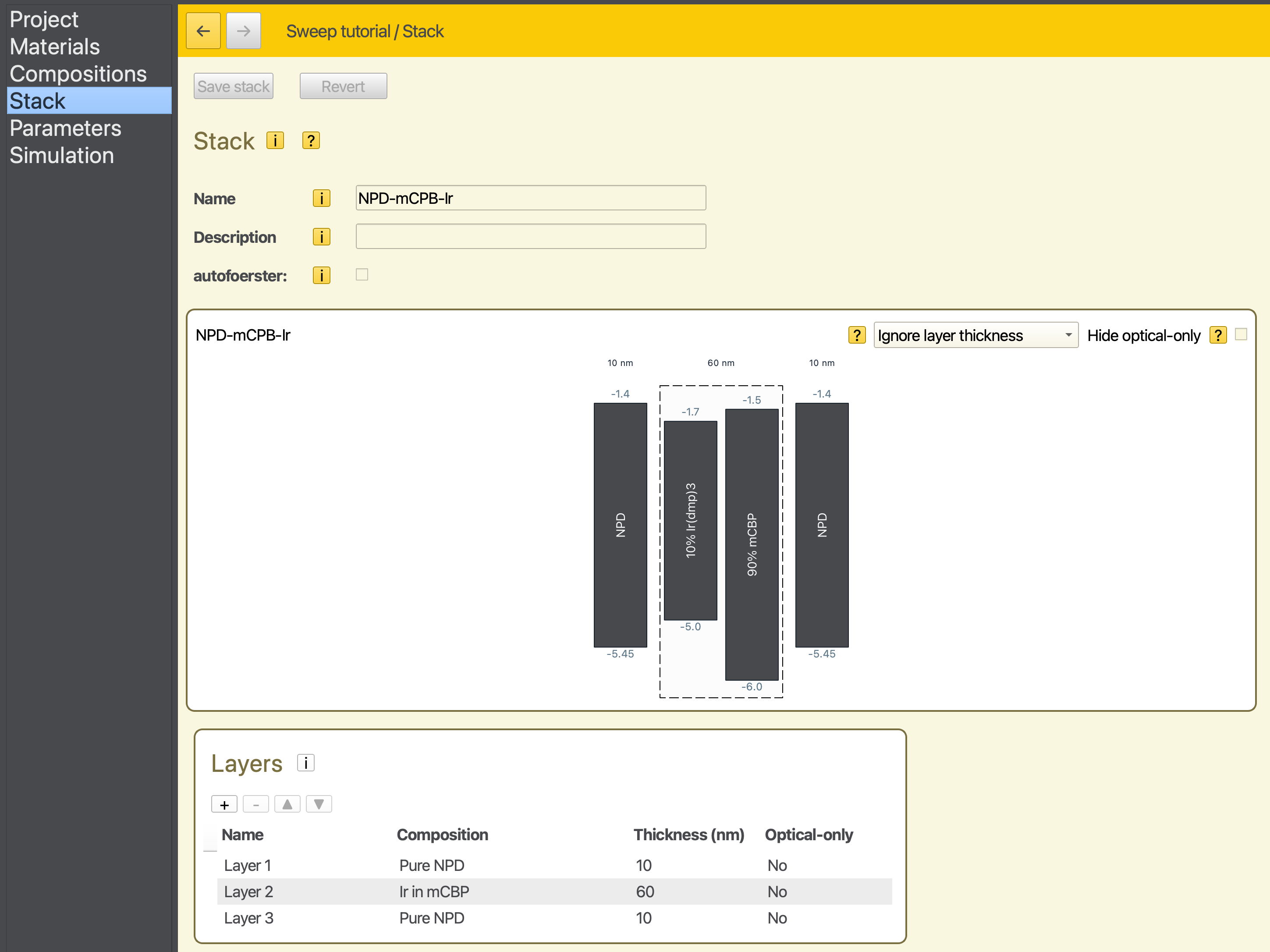
Fig. 26 Diagram of the OLED device
Create a Parameter Set
For this simulation, we are interested in investigating the device performance at different voltages. Click on the Load preset button and select the Voltage sweep (bipolar) template:
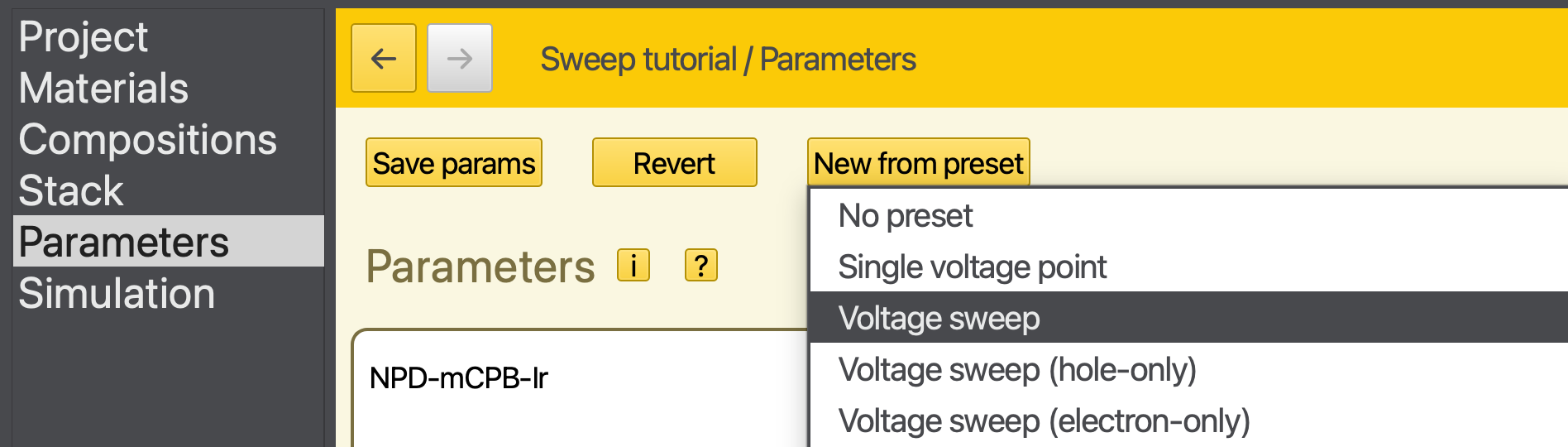
Fig. 27 Template selection for the parameter set
The voltage will be set as part of the parameter screening and does not need to be chosen at this step.
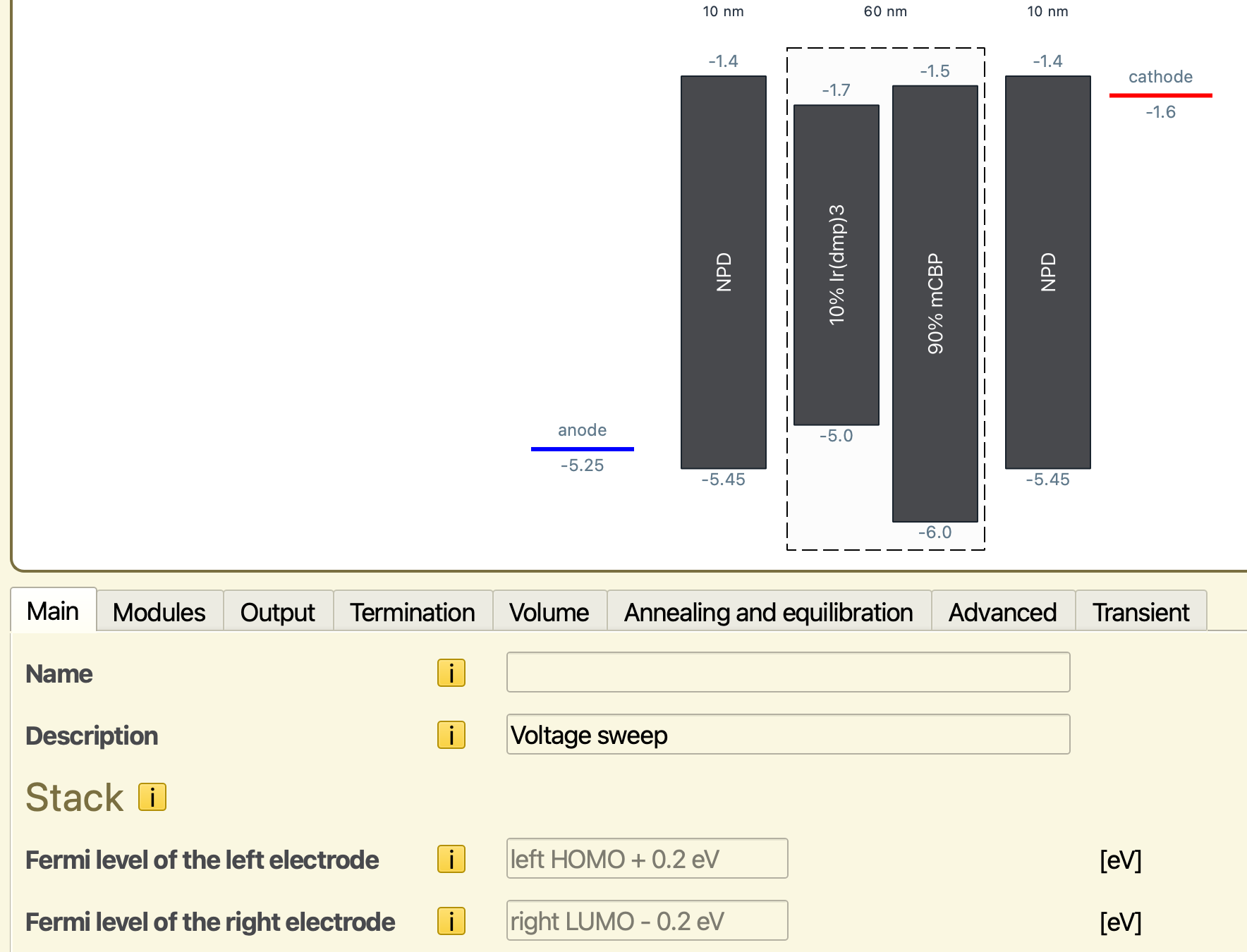
Fig. 28 Electrode contacts are configured automatically to include an exchange barrier
The Fermi levels of the electrodes are automatically matched to the material parameters. These levels can be adjusted to those of the external contacts. We will use an electrode energy level of -5.25 at the anode and -1.6 at the cathode. By using an energy barrier of 0.2 eV compared to the NPD polaron energy levels, we are reducing the rate of polaron exchange processes with the electrodes. This biases the kMC simulation, increasing the number of samples that contain transport processes compared to electrode exchange.
Note
Care should be taken that this artificial barrier does not affect the device statistics. This can be achieved by analyzing the change in device properties when varying the barrier height. Because electrode exchange processes are localized at the edges of the device, a single-layer simulation can be used to perform these screenings, significantly reducing the simulation costs.
For simulations conducted at typical OLED voltages, the default 0.2 eV barrier is typically sufficient.
Note
When operating under high currents, the device sensitivity to the barrier height may become voltage-dependent. Make sure to verify the validity of your data at both extremities of the investigated voltage range.
The Modules tab allows you to enable different processes that are allowed to occur during the simulation. We disable the excitonics module, as we will exclusively focus on polaron transport for this tutorial.
We set the number of simulation steps to 10,000,000 in the Termination tab. On the Output tab, we set the report interval to 100,000 and the output interval to 500,000. The parameter set can now be saved by pressing the Save parameters button.
Starting the Simulation
Navigate to the Simulation page. For this tutorial, we set the number of trajectories to 1 in order to reduce the required number of processors. This will generate 1 trajectory per voltage point.
Parameter screenings can be specified as part of the simulation setup. The screening allows evaluation of the device behavior for different parameter values. Aside from the sweep parameter, all other conditions will remain unaltered from the default parameter set.
The screening values are obtained through linear interpolation. Minimum and maximum values for the screening parameter are selected and the total number of screening steps is chosen. A uniform step size between parameter values is calculated.
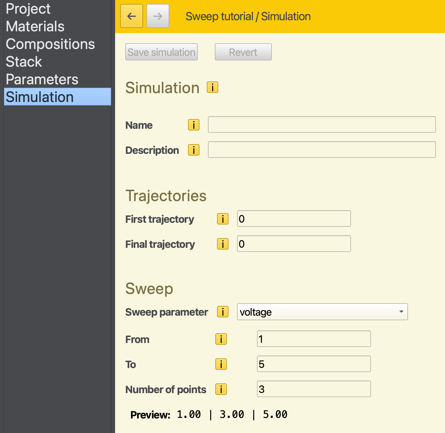
Fig. 29 Voltage sweep setup in the simulation settings
For this example, we select the voltage as our screening parameter. The minimum and maximum voltages are set to 1 and 5 V respectively. By choosing 3 voltage steps, this will prompt the screening to perform simulations at 1, 3 and 5 V. A preview of these screening conditions is provided in the interface.
Note that trajectories are generated at each screening step. The default of 5 trajectories would therefore yield 15 independent jobs. By using only a single trajectory instance, the number of simulation jobs is limited to 3.
We now save our project (File → Save) which will automatically set up a new simulation in AMSjobs. You can start the simulation by selecting File → Run.
We wait for the screening steps to complete. In the meantime, we can monitor the progress of the simulation with BBresults.
Simulation Output
We can visualize the output of the (ongoing) simulation using BBresults. Select SCM → BBresults either from AMSjobs or BBinput to view the results of our voltage sweep.
The convergence of the simulations at each voltage point can be viewed from the main Status page. We see that the convergence of the low-voltage simulations proceeds more slowly.
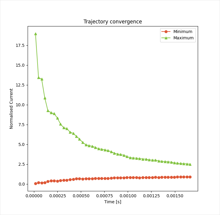
Fig. 30 Convergence of the transient device current at 3 V
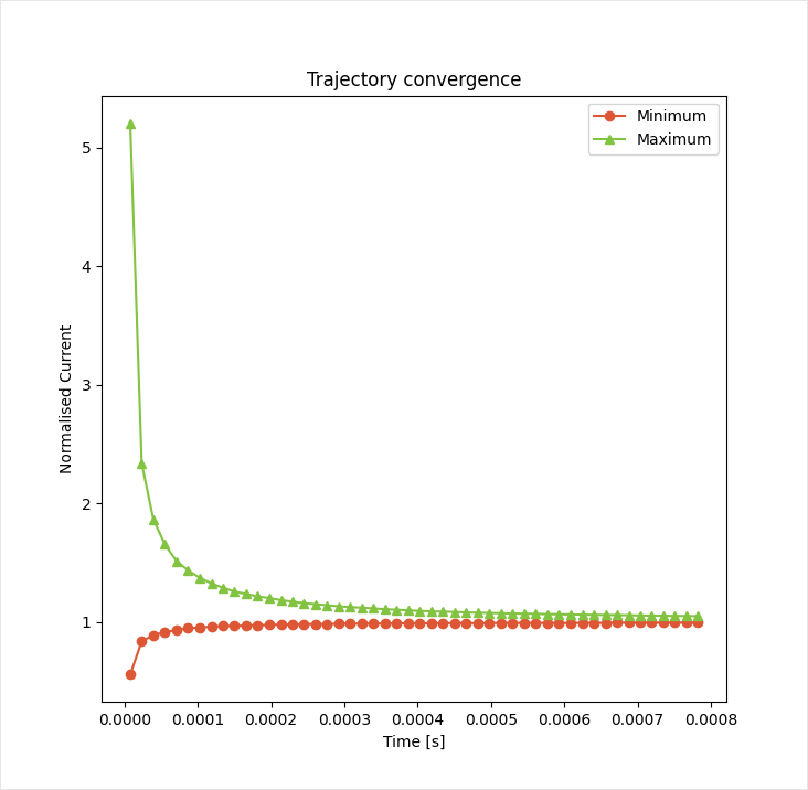
Fig. 31 Convergence of the transient device current at 5 V
A lower driving voltage reduces the mobility of the charge carriers. It takes a longer time before the charges move from the electrodes into the emissive layer. This process can be seen from the carrier profiles under Device → Profiles → Electron Density per Voltage.
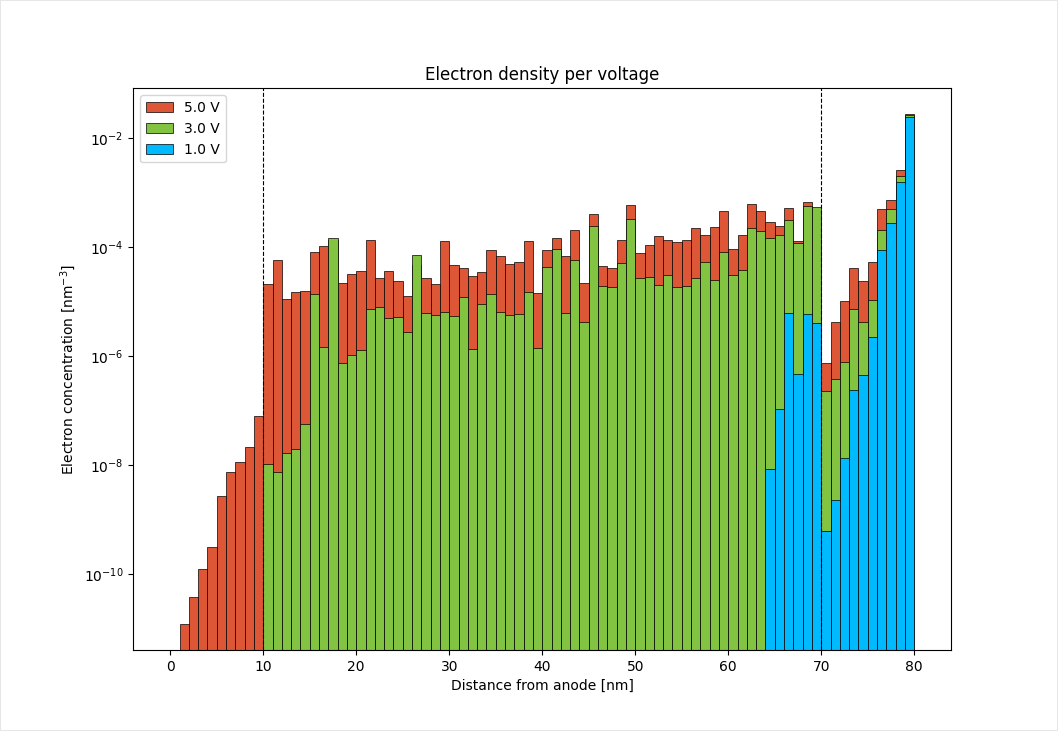
Fig. 32 Electron concentration profile over the NPD-OLED device. Dashed lines indicate the layer boundaries
Current-voltage characteristics can be viewed in the Device → Overview → Current-Voltage Profile.
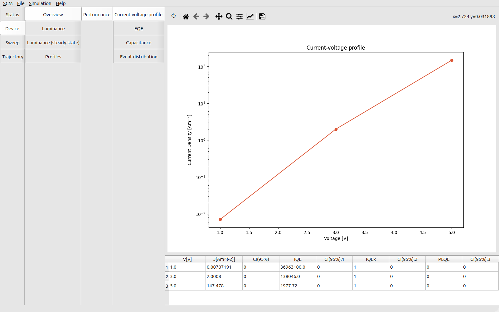
Fig. 33 Simulated JV profile of the NPD-OLED device
Extending the Simulation Time
Because low-voltage simulations converge slowly, it is possible that the number of simulation steps is not enough to reach the steady-state.
In BBresults, it is possible to extended the duration of a simulation by adding additional simulation time. Once the simulation has finished, the Simulation → Extend trajectories option can be used to restart Bumblebee.
Note
Restart files must have been enabled in the Output section of the Parameters page.
This is true by default, though users may choose to forgo writing these files in order to reduce the amount of data that is written to disk.
Note
When using a remote queue with a job scheduler (such as SLURM), is it possible that the simulation will time out before the maximum number of steps is reached.
In this case, extending a trajectory will restart from the last state that was recorded in the output.
Extending the Voltage Range
After performing an initial screening, it is possible to add additional sample points. From BBresults, the Simulation → Add sweep point option can be used to request additional jobs. The output from these jobs is then automatically collected and appended to the current simulation. This option was used in the previous tutorial to improve simulation statistics, but can also be used to extend the sweep range or to add additional points to the parameter screening.
For this tutorial, we will extend the voltage range. In Simulation → Add sweep point we request a voltage sweep from 1.0 to 7.0 V using 7 steps.
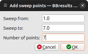
Press the OK button. The Status page in BBresults will now update with the extended parameter sweep:
The resolution of the screening is increased by adding two new screening points at 2.0 V and 4.0 V. The simulations at 1.0 V, 3.0 V and 5.0 V are skipped as they are already part of the parameter sweep.
The voltage range has been extended with 2 new voltage points at 6.0 V and 7.0 V.
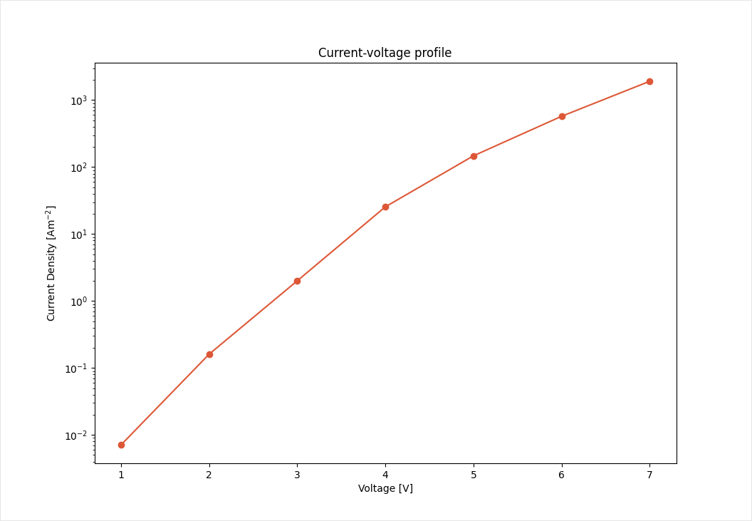
Fig. 34 Simulated JV profile for the extended parameter sweep