Automated PES Exploration¶

In chemistry and materials science, two types of Potential Energy Surface (PES) critical points are of particular interest: local minima and (first-order) saddle points.

The PESExploration task consists of a set of algorithms (which we will refer to as jobs) that will automatically explore the PES of a given system, looking for local minima and saddle points.

The available PES exploration jobs are:

Process Search: A composite method for finding escape mechanisms from a state. This will find both local minima and saddle points.
Basin Hopping: A Monte Carlo method for finding local minima.
Saddle Search: A single-ended method for finding nearby saddle points.
Landscape Refinement: Given a pre-calculated Energy Landscape, re-optimize local minima and saddle points using a different computational engine/settings.
Binding Sites: Given a pre-calculated Energy Landscape, compute the binding sites.

The AMS driver links to the client program of the EON software package 1 and uses its implementation of the dimer method. EON is developed by the University of Texas at Austin and the University of Iceland. See also the Required citations section.

See also

PES Exploration GUI tutorials:
Examples:

Tip

There is a separate tool specifically for the generation of conformers, see this manual page. While the PES exploration can in principle also be used to find conformers, using the dedicated Conformers tool is usually easier and faster. Note that the set of minima found by the Conformers tool can be used as input for a PES exploration, see this example.

Overview¶

While many details of a PES exploration calculation depend on the specific job selected, some aspects are common to all PES explorations jobs. Here we give a brief overview of a typical PES exploration, using a Process Search job as example.

A PES exploration calculation generally consists of multiple expeditions, each with several explorers.

Explorers are given an initial structure, and their goal is to find a nearby critical point (a local minimum, a saddle point or both). The explorer moves around the PES by modifying the atomic positions of the system and by using the specified Engine to compute energy and gradients.

An expedition is a collection of explorers all starting from the same point on the PES.

Before setting off for the first expedition, the input structure is optimized and added to the Energy Landscape, which is the database of all interesting points found during the exploration (see the section Results: the “Energy Landscape” for more details).

Starting from this initial structure, a number of PES explorers (3 in the diagram below) will set off in random directions exploring the potential energy surface and looking for nearby critical points.

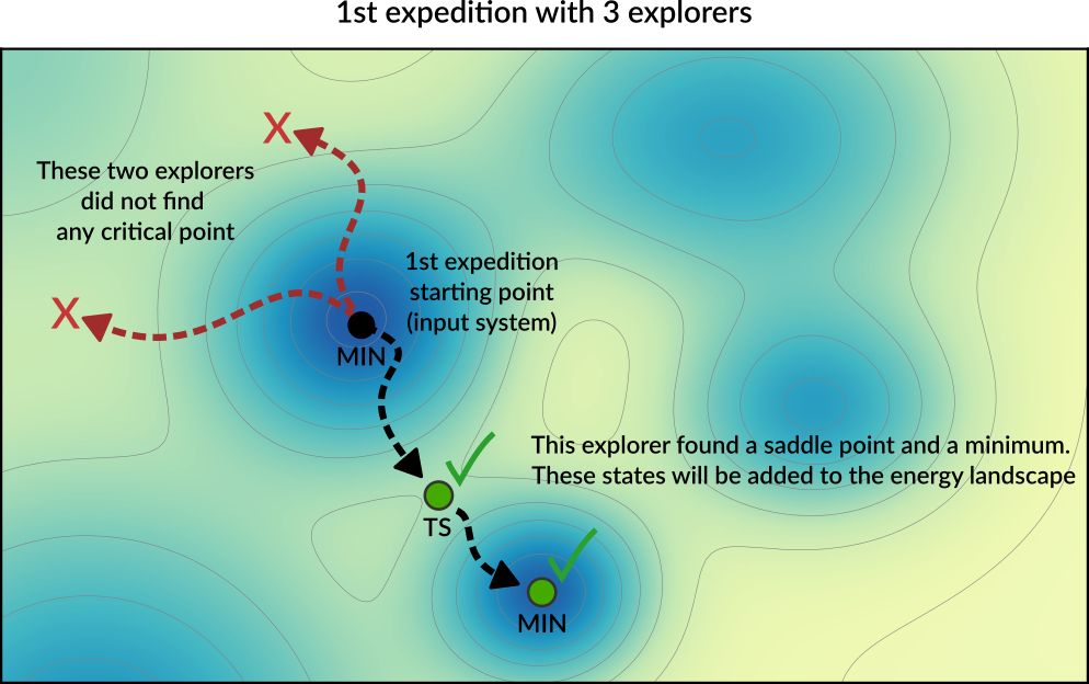
Explorers have “stop conditions” (e.g. a maximum number of steps or a maximum energy above the starting point) so in general not all explorers will successfully find a critical point. In this case, only one of the explorers found relevant critical points: a saddle point and a local minimum. These newly found critical points are added to the Energy Landscape.

After the first expedition is over, the program will start with the second expedition. The starting point for the next expedition will be a randomly chosen local minimum from the list of minima present in the Energy Landscape (the possible starting points for an exploration are called seed states. See also the DynamicSeedStates option).

In this example, the starting point of the second expedition is the new local minimum found during the first expedition. A new set of explorers will set off in random directions from this point.

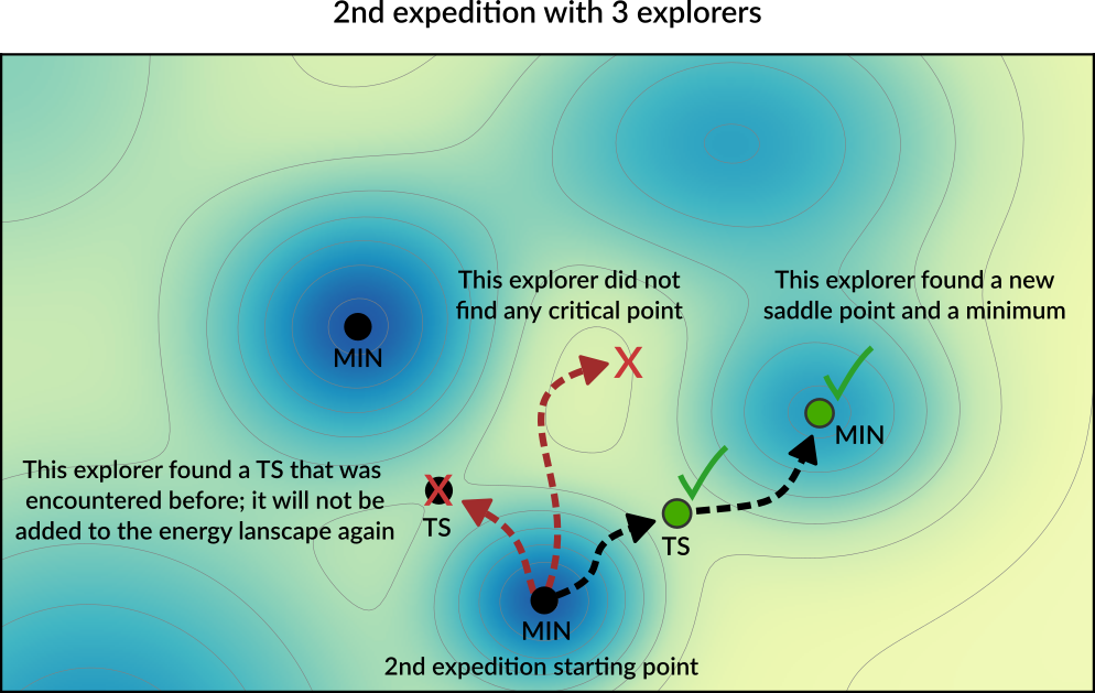
In the diagram above, one of the explorer found a saddle point that was already found in a previous exploration. This structure will not be added to Energy Landscape since it was already seen before (see the Structure comparison section for more details). The newly found critical points are added to the Energy Landscape.

Usually, many expeditions and/or many explorers are needed to map the PES, but you should keep in mind that the computation time of the calculation will roughly be proportional to the product NumExpeditions x NumExplorers.

By having many explorers you will have a higher chance of comprehensively mapping the PES near the starting point of each expedition. By having many expeditions, you will have a higher chance of traveling further away from the initial structure.

It should be emphasized that the PES exploration task is stochastic in nature, as it uses random numbers to perform initial-displacements. This means that if you run the same calculation twice you might find different critical points.

Job selection and main options¶

To use one of the PES Exploration procedures you should set the Task to PESExploration and specify one of the jobs in the PESExploration%Job key:

Task PESExploration

PESExploration
   Job [ProcessSearch | BasinHopping | SaddleSearch | LandscapeRefinement | BindingSites]
End

The input options for the various jobs are described in the corresponding sections: Process Search, Basin Hopping, Saddle Search, Landscape Refinement, Binding Sites.

It is then important pick an appropriate number of expeditions and explorers. Having many expeditions and explorers will result in a more comprehensive PES exploration, but since the computation time will roughly be proportional to the product NumExpeditions x NumExplorers you’ll need to find an appropriate balance.

PESExploration
   NumExpeditions integer
   NumExplorers integer
   DynamicSeedStates Yes/No
End

PESExploration

Type: Block
Description: Configures details of the automated PES exploration methods.

NumExpeditions

Type: Integer
Default value: 1
Description: Sets the number of subsequent expeditions our job will consist of. Larger values result in a more comprehensive exploration of the potential energy surface, but will take more computational time.

NumExplorers

Type: Integer
Default value: 1
Description: Sets the number of independent PES explorers dispatched as part of each expedition. Larger values will result in a more comprehensive exploration of the potential energy surface, but will take more computational time. By default an appropriate number of explorers are executed in parallel.

DynamicSeedStates

Type: Bool
Default value: Yes
Description: Whether subsequent expeditions may start from states discovered by previous expeditions. This should lead to a more comprehensive exploration of the potential energy surface. Disabling this will focus the PES exploration around the initial seed states.

The following miscellaneous input option generally apply to most PES exploration calculations:

PESExploration
   WriteHistory [None | Converged | All]
   Temperature float
   FiniteDifference float
End

PESExploration

Type: Block
Description: Configures details of the automated PES exploration methods.

WriteHistory

Type: Multiple Choice
Default value: Converged
Options: [None, Converged, All]
Description: When to write the molecular geometry (and possibly other properties) to the history on the ams.rkf file. The default is to only write the converged geometries to the history. Can be changed to write no frames at all to the history, or write all frames (should only be used when testing because of the performance impact). Note that for parallel calculations, only the first group of processes writes to ams.rkf.

Temperature

Type: Float
Default value: 300.0
Unit: Kelvin
Description: The temperature that the job will run at. This may be used in different ways depending on the job, e.g. acceptance probabilities for Monte-Carlo based jobs, thermostatting for dynamics based jobs, kinetic prefactors for jobs that find transition states. Some jobs may not use this temperature at all.

FiniteDifference

Type: Float
Default value: 0.0026458861
Unit: Angstrom
Description: The finite difference distance to use for Dimer, Hessian, Lanczos, and optimization methods.

Results: the “Energy Landscape”¶

The results of a PES Exploration are the structures and energies of the critical points found. There are multiple ways for you to inspect the results:

The energy landscape can be visualized using the AMSMovie GUI module (In AMSMovie: File → Open and select the ams.rkf file of your calculation). See the GUI tutorials (e.g. Automated reaction pathway discovery for hydrohalogenation) for more details.
The results are printed to the text output under the header Final Energy Landscape, see below.
The results are stored on the ams.rkf binary results file in the section EnergyLandscape
In PLAMS, you can use the get_energy_landscape method of the AMSResults object to conveniently extract the results.

Results on the text output¶

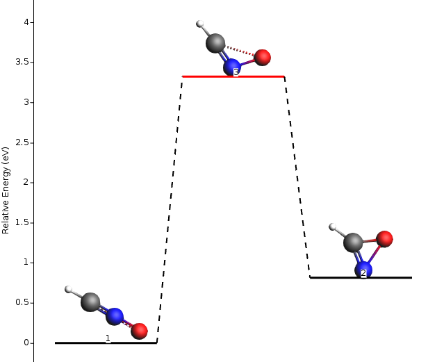
These are printed at the end of the text output under the header Final Energy Landscape. Here is an output example for a ProcessSearch job for the simple HCN molecule (computed with the DFTB engine):

----------------------
Final Energy Landscape
----------------------

      Id        Energy(a.u.)         RE(eV)   RE(kcal/mol)    Counts    Crit. point
   --------------------------------------------------------------------------------
       1           -5.782789        0.00000         0.0000         4            Min
       2           -5.748792        0.92510        21.3334         4            Min
       3           -5.689025        2.55143        58.8375         4             TS  1 <--> 2

Number of configurations                             3
Number of local minima                               2
Number of transition states                          1
Energy range (a.u.)                           0.093763
Energy range (eV)                              2.55143
Energy range (kcal/mol)                        58.8375

Configurations
--------------
3
Id 1 Energy(hartree)     -5.78278852 isTS=False
H       -5.05604362312999       1.04394551246415       0.36836337958238
C       -4.06812264817497       0.95005534859126      -0.01533183100739
N       -3.00601476684712       0.84907755770632      -0.42810754191928
3
Id 2 Energy(hartree)     -5.74879169 isTS=False
H       -4.01886309319822       1.09046314142766       1.01610923624838
C       -4.06910389782095       0.79751242545583      -1.12016730790896
N       -4.04221404713293       0.95510285187825       0.02898207831626
3
Id 3 Energy(hartree)     -5.68902502 isTS=True
H       -4.51488871821561       1.04261603660424       0.52096081259126
C       -4.32990923520194       0.88203060069718      -0.58636688911847
N       -3.28538308473452       0.91843178146029      -0.00966991681712

From this you can see that 3 critical points were found: 2 minima (Id 1 and Id 2) and 1 transition state (Id 3) connecting the first two states (indicated by 1 <--> 2).

Under Counts you can see how many times each state was encountered during the exploration (often the same state is found multiple times) See the Structure comparison section for more details on how states are compared.

RE is the “relative energy” with respect to the lowest-energy state found.

Under the header Configurations you will find the XYZ geometries (in Angstrom) corresponding to the various critical points.

Continue a PES exploration from a previous calculation¶

You can load an Energy Landscape obtained from a PES exploration calculation (or by the Conformers utility) and use it as starting point for a new PES exploration. In this way you can extend your Energy Landscape, and potentially use different PES exploration algorithms.

To load a previously computed energy landscape, use the PESExploration%LoadEnergyLandscape%Path option (note: you should still provide an input system in the System block even if you are loading a previous Energy Landscape. The input system will be optimized and added to the energy landscape as a minimum).

It is often convenient to load only some of the states from a previous calculation; this can be done via the Remove or KeepOnly input options. Specify the seed states with the SeedStates option.

These are all the input options related to the loading an Energy Landscape:

PESExploration
   LoadEnergyLandscape
      GenerateSymmetryImages Yes/No
      KeepOnly integer_list
      Path string
      Remove integer_list
      RemoveWithNoBindingSites Yes/No
      SeedStates integer_list
   End
End

PESExploration

LoadEnergyLandscape

Type: Block
Description: Options related to the loading of an Energy Landscape from a previous calculation.

GenerateSymmetryImages

Type: Bool
Default value: No
Description: By activating this option, after loading the energy landscape, it will create the complete set of symmetry-related copies by using the symmetry operators of the reference structure. Be aware that rkf result files of the generated symmetry images are copies from the parent structures but only atomic coordinates are updated.

KeepOnly

Type: Integer List
GUI name: List of states to keep
Description: Upon loading the Energy Landscape, only keep the states specified here. The states should be specified via a list of integers referring to the indices of the states you want to keep.

Path

Type: String
GUI name: Load energy landscape from
Description: AMS results folder to load an energy landscape from. In the text input file, you may alternatively specify a .con file in the native EON format.

Remove

Type: Integer List
GUI name: List of states to remove
Description: Upon loading the Energy Landscape, remove (i.e. do not load) the states specified here. The states should be specified via a list of integers referring to the indices of the states you want to remove (i.e. the states you don’t want to load).

RemoveWithNoBindingSites

Type: Bool
Default value: No
Description: Upon loading the Energy Landscape, it removes states with no associated binding sites. Associated transition states are also removed. This is an advantageous option to remove physisorbed states automatically. Notice that it requires that the previous calculation was executed, enabling the option [BindingSites%Calculate].

SeedStates

Type: Integer List
GUI name: List of seed states
Description: By default when you start a new PES Exploration from a loaded Energy Landscape, expeditions can start from any of the loaded minima. By using this input option, you can instruct the program to only use some of the states as ‘expedition starting point’. The states that serve as ‘expedition starting points’ should be specified via a list of integers referring to the indices of the states.

Troubleshooting¶

The PES exploration in AMS is quite sensitive to noise on the potential energy surface. A too noisy PES may result in bad convergence of the individual explorers, or states being rejected because their PES point character is not the expected one.

In case of problems we therefore advise to set engine options that result in a smoother PES. Often this can be accomplished by setting the NumericalQuality keyword in the engine input.

Especially the ReaxFF engine has a rather noisy PES by default, which may cause problems in a PES exploration job. Please refer to the ReaxFF manual for advice on how to smoothen the ReaxFF potential energy surface:

Structure comparison¶

During a PES exploration some critical points will most likely be encountered more than once.

Whenever a critical point is found, the program will ask itself: is this a new structure, or have I already encountered this before? If the structure was not seen before (i.e. it’s a novel configuration), it will be added to the list of structures found during the exploration. If the structure was already found before, the program will simply increase a counter keeping track of how many times a specific structure was found during the PES exploration.

When deciding if two structures are the same or not, the program will compare both the geometry and the energy of the two configurations. Several parameters and thresholds can be tweaked in the PESExploration%StructureComparison block to tell AMS under which conditions two systems should be considered equal.

PESExploration
   StructureComparison
      CheckRotation Yes/No
      CheckSymmetry Yes/No
      DistanceDifference float
      EnergyDifference float
      IndistinguishableAtoms Yes/No
      NeighborCutoff float
      RemoveTranslation Yes/No
   End
End

PESExploration

StructureComparison

Type: Block
Description: Settings for structure comparison.

CheckRotation

Type: Bool
Description: Rotates the system optimally before comparing structures. The default is to do this only for molecular systems when there are no fixed atom constraints.

CheckSymmetry

Type: Bool
Default value: No
Description: Considers that two systems are equal if they are equivalent by symmetry.

DistanceDifference

Type: Float
Default value: 0.1
Unit: Angstrom
Description: If the distance between two mapped atoms is larger than this threshold, the two configurations are considered different structures.

EnergyDifference

Type: Float
Default value: 0.01
Unit: eV
Description: If the energy difference between two configurations is larger than this threshold, the two configurations are considered to be different structures.

IndistinguishableAtoms

Type: Bool
Default value: Yes
Description: If yes, the order of the atoms does not affect the structural comparison. Atoms of the same element are then indistinguishable.

NeighborCutoff

Type: Float
Default value: 3.3
Unit: Angstrom
Description: Atoms within this distance of each other are considered neighbors.

RemoveTranslation

Type: Bool
Description: Translates the system optimally before comparing structures. The default is to do this only when there are no fixed atom constraints.

Process Search job¶

Overview¶

Process Search is a composite method for finding escape mechanisms from a state. Each PES explorer will perform the following steps:

Starting from a minimum, a SaddleSearch calculation is performed to find a nearby saddle point
If a saddle point is found, two images are placed on either side of the saddle along the min mode.
The two images are then minimized; one of the images is expected to fall back into the original minimum, while the other image is expected to end up in the product state on the other side of the saddle. If this is case, the product, TS and reactant states are added to the energy landscape.

The Process Search procedure will therefore not only find minima and saddle points, but it will also keep track of which minima each saddle point is connecting.

See also

GUI tutorials Automated reaction pathway discovery for hydrohalogenation and Water dissociation on an oxide surface.

Input options¶

To perform a Process Search calculation you should specify:

Task PESExploration

PESExploration
   Job ProcessSearch

   ProcessSearch
      # Options for the Process Search procedure. See description below.
   End

   SaddleSearch
      # Options for the Saddle Search part of the Process Search procedure.
   End
End

The options for the saddle search part of a Process Search job are described in the SaddleSearch section.

Options specific to the Process Search procedure can be specified in the PESExploration%ProcessSearch block:

PESExploration
   ProcessSearch
      MinimizationOffset float
   End
End

PESExploration

ProcessSearch

Type: Block
Description: Input options specific to the process search procedure.

MinimizationOffset

Type: Float
Default value: 0.2
Description: After a saddle is found, images are placed on either side of the saddle along the mode and minimized to ensure that the saddle is connected to the original minimum and to locate the product state. MinimizationOffset is the distance those images are displaced from the saddle.

Saddle Search job¶

Overview¶

Saddle Search is a single-ended method for finding nearby saddle points.

In a Saddle Search calculation, each PES explorer starts by performing a random displacement from the initial geometry (or seed state). Then, starting from this point, the explorer searches for a nearby saddle point using a minimum-mode following method (the available min-mode following methods are dimer 3 4 5 and Lanczos 6).

If you already know which atoms are likely to be involved in the reactions, you can use the DisplaceAtomsInRegion option to nudge the Saddle Search procedure towards the right part of the PES (regions can be specified in the system input block, or via the “Model → Regions” panel in AMSinput).

Input options¶

To perform a Saddle Search calculation you should specify:

Task PESExploration

PESExploration
   Job SaddleSearch

   SaddleSearch
      # Options for the Saddle Search procedure. See description below.
   End
End

Options for the Saddle Search procedure can be specified in the PESExploration%SaddleSearch block.

Note: these options also affect the Saddle Search part of Process Search Jobs.

PESExploration
   SaddleSearch
      ConvergedForce float
      DisplaceAlongNormalModesActiveModes string
      DisplaceAlongNormalModesWeight float
      DisplaceAtomsInRegion string
      DisplaceAtomsInRegionWeight float
      DisplaceListedAtoms string
      DisplaceListedTypes string
      DisplaceMagnitude float
      DisplaceRadius float
      MaxEnergy float
      MaxIterations integer
      MinEnergyBarrier float
      MinModeMethod [dimer | lanczos]
      RelaxFromSaddlePoint Yes/No
      ZeroModeAbortCurvature float
   End
End

PESExploration

SaddleSearch

Type: Block
Description: Configuration for the Saddle Search procedure (used in SaddleSearch and ProcessSearch Jobs).

ConvergedForce

Type: Float
Default value: -1.0
Unit: eV/Angstrom
Description: Convergence threshold for nuclear gradients. Note: Special value of -1.0 means using the same convergence criterion as the PES explorer’s geometry optimizer.

DisplaceAlongNormalModesActiveModes

Type: String
Default value
Description: Sets the active modes to be used when the option [SaddleSearch%DisplaceAlongNormalModesWeight] is enabled. e.g. 1,2,3,5. By default, all normal modes are considered active.

DisplaceAlongNormalModesWeight

Type: Float
Default value: 0.0
Description: The probability of generating a displacement resulting in a random linear combination of the normal modes specified in [SaddleSearch%DisplaceAlongNormalModesActiveModes]. This parameter is a numeric value that should fall within the interval [0.0, 1.0].

DisplaceAtomsInRegion

Type: String
Default value
Description: A string corresponding to the name of a region. When performing the initial random displacement, only displace atoms in the specified region.

DisplaceAtomsInRegionWeight

Type: Float
Default value: 0.0
Description: The probability of generating a displacement involving only atoms from the region specified in [SaddleSearch%DisplaceAtomsInRegion]. This parameter is a numeric value that should fall within the interval [0.0, 1.0].

DisplaceListedAtoms

Type: String
Default value
Description: Sets the active atoms to be used when the option [SaddleSearch%DisplaceAlongNormalModesWeight] is enabled. e.g. 1,2,3,5. By default, all normal modes are considered active.

DisplaceListedTypes

Type: String
Default value
Description: ???.

DisplaceMagnitude

Type: Float
Default value: 0.1
Unit: Angstrom
Description: The standard deviation of the Gaussian displacement in each degree of freedom for the selected atoms.

DisplaceRadius

Type: Float
Default value: 4.0
Unit: Angstrom
Description: Atoms within this distance of the epicenter will be displaced.

MaxEnergy

Type: Float
Default value: 20.0
Unit: eV
Description: The energy (relative to the starting point of the saddle search) at which a saddle search explorer considers the search bad and terminates it.

MaxIterations

Type: Integer
Default value: 400
Description: Maximum number of iterations for each saddle search run.

MinEnergyBarrier

Type: Float
Default value: 0.001
Unit: eV
Description: Minimum energy barrier to accept a new transition state.

MinModeMethod

Type: Multiple Choice
Default value: dimer
Options: [dimer, lanczos]
Description: The minimum-mode following method to use.

RelaxFromSaddlePoint

Type: Bool
Default value: No
Description: Relaxes the saddle point geometries following the imaginary mode to get both reactants and products.

ZeroModeAbortCurvature

Type: Float
Default value: 0.01
Unit: eV/Angstrom^2
Description: The threshold in the frequency below which the minimum mode is considered zero. The calculation is aborted if the negative mode becomes zero.

Basin Hopping job¶

Overview¶

Basin hopping 2 is an iterative Monte Carlo method for PES exploration and global minimization.

An “iteration” in basin hopping consists of the following steps:

The atomic coordinates of the system are randomly perturbed (the details of this random perturbation can be configured via the keywords Displacement, DisplacementDistribution, SingleAtomDisplace, SwapProbability. See below for more details).
A local optimization of the randomly perturbed structure is performed (see also the Optimizer section)
The new optimized structure is accepted or rejected based of its energy (if the energy of the newly optimized structure lower than the lowest energy so far, the new structure is readily accepted. Otherwise it is accepted with probability \(e^{(-\Delta E / kT)}\) where \(\Delta E\) is the difference between the energy at the previous iteration and the current energy, \(T\) is temperature specified in the PESExploration%Temperature keyword, see Job selection and main options).

By iteratively performing these steps, the basin hopping procedure explores the highly-dimensional configuration space of the system, looking for the global minimum and finding local minima along the way. The number of iteration can be specified via the Steps keywords (see below for more details).

For a more comprehensive PES exploration, AMS can perform several expeditions (potentially with several explorers for each expedition) in a single calculation. See the NumExpeditions and NumExplorers keywords in the Job selection and main options section for more details.

See also

Example: Basin Hopping for Ar 13 cluster
GUI tutorials Cluster Growth: Cobalt Clusters and Water dissociation on an oxide surface.

Input options¶

To perform a Basin Hopping calculation you should specify:

Task PESExploration

PESExploration
   Job BasinHopping

   Temperature float

   BasinHopping
      # Options for the Basin Hopping procedure. See description below.
   End
End

The PESExploration%Temperature keyword is described in the Job selection and main options section.

The following input keywords are specific to Basin Hopping procedure:

PESExploration
   BasinHopping
      DisplaceAtomsInRegion string
      Displacement float
      MainSystemAsSeed Yes/No
      PESPointCharacterization Yes/No
      PushApartDistance float
      Steps integer
   End
End

PESExploration

BasinHopping

Type: Block
Description: Configures the details of the Basin Hopping subtask.

DisplaceAtomsInRegion

Type: String
Default value
Description: If you specify a region name here, only the atoms belonging to this region will be displaced during the basin hopping procedure. For more details on regions, see the documentation on the System definition.

Displacement

Type: Float
Default value: 0.5
Unit: Angstrom
Description: Displacement in each degree of freedom.

MainSystemAsSeed

Type: Bool
Default value: No
Description: If true, only the main system will be used as a seed state. The main system is not added to the database.

PESPointCharacterization

Type: Bool
Default value: Yes
Description: If true, a PES point characterization based on a vibrational analysis is carried out to confirm each detected state is an actual local minimum (no imaginary frequencies). Conversely, if this option is false, the PES point characterization is avoided, which will assume that all located states are local minima (zero gradients). Enabling this option is very useful for large systems. It circumvents the need for computing and diagonalizing the Hessian matrix, a typically expensive computational process.

PushApartDistance

Type: Float
Default value: 0.4
Unit: Angstrom
Description: Push atoms apart until no atoms are closer than this distance. This criterion is enforced for the initial structure and all those generated by random displacements.

Steps

Type: Integer
Default value: 20
Description: Number of displace & optimize Monte-Carlo steps to take.

Fragmented states¶

When studying adsorption processes, it is required to review those situations where a transition state (TS) does not mediate the adsorption process. They are formally known as non-activated exothermic adsorption processes. These processes are not discovered naturally in the PES exploration. Since the AMS2022 release, there is a systematic way of including those processes. To this aim, we defined the fragmented states, where the adsorbate and adsorbent are infinitely far away from each other.

The fragmented states can be included in the Energy Landscape through the use of the CalculateFragments keyword:

PESExploration
   CalculateFragments Yes/No
End

PESExploration

CalculateFragments

Type: Bool
Default value: No
Description: Must be used together with an adsorbent set as the StatesAlignment%ReferenceRegion. Runs a final calculation of the adsorbate and adsorbent (marked by the ReferenceRegion) individually. The fragmented state is included in the energy landscape.

The keyword has to be used together with a reference region set via the StatesAlignment%ReferenceRegion keyword. The calculation of the fragmented states will happen at the very end of a PES exploration. For every minimum in the energy landscape, two geometry optimizations will be performed: one with only the atoms belonging to the reference region (the adsorbent), the other with only the atoms outside of the reference region (the adsorbate). This relaxes the structure of the adsorbent in the absence of the adsorbate, and vice versa.

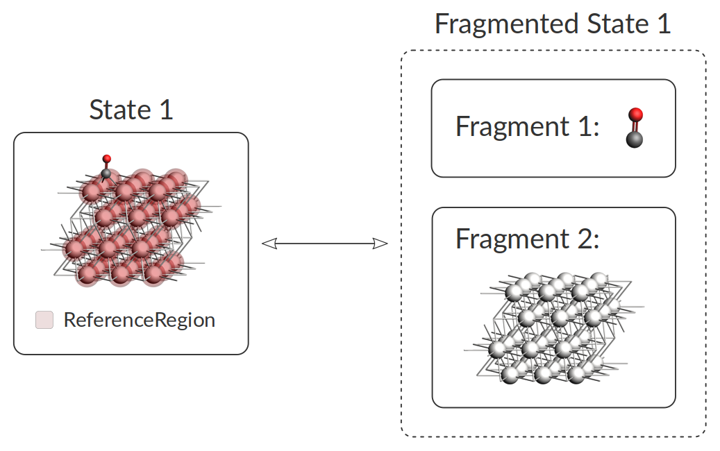
The total energy of the fragmented state is then simply taken as the sum of the energies of both fragments, and the adsorption energy is the difference between the adsorbed and fragmented state.

\[\begin{split}E\big(\text{fragmented state 1}\big) = E\big(\text{fragment 1}\big) + E\big(\text{fragment 2}\big) \\ E_{ad} = E\big(\text{state 1}\big) - E\big(\text{fragmented state 1}\big)\end{split}\]

You will find fragmented states and the fragments in the text output following the Final Energy Landscape section. The example shown above would look like this:

----------------------
Final Energy Landscape
----------------------

        Id        Energy(a.u.)         RE(eV)   RE(kcal/mol)    Counts    Crit. point
     --------------------------------------------------------------------------------
         1           -7.651642        0.00000         0.0000         1            Min
         2           -7.651572        0.00191         0.0441         1            Min
         3           -7.623820        0.75709        17.4589         1            Min
         4           -7.622548        0.79170        18.2571         7             TS 2<-->3
         5           -7.622430        0.79491        18.3310         5             TS 3<-->1

Number of configurations                             5
Number of local minima                               3
Number of transition states                          2
Energy range (a.u.)                           0.029212
Energy range (eV)                              0.79491
Energy range (kcal/mol)                        18.3310

Fragments
---------

Number of fragments                                  2

        Id             Formula        Energy(a.u.)              Region
     -----------------------------------------------------------------
         1                  CO           -0.424454              active
         2                Pt36           -7.154286             surface

Fragmented States
-----------------

Number of fragmented states                          1

        Id           Fragments        Energy(a.u.)         RE(eV)   RE(kcal/mol)
     ---------------------------------------------------------------------------
         1                 1,2           -7.578740        1.98377        45.7467 -->1
                                                                                 -->2
                                                                                 -->3

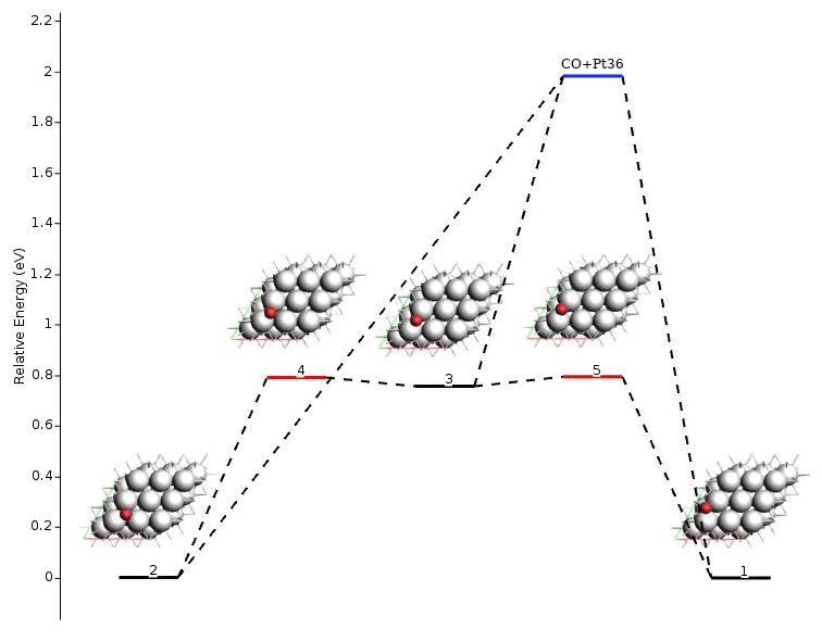
Notice the following: 1) one fragment may be included in multiple fragmented states, and 2) multiple states may be connected to the same fragmented state. The latter happens when the individual optimizations of adsorbate and adsorbent yield the same results for multiple states. By definition, these states are considered connected if the difference in energy is lower than PESExploration%SaddleSearch%MaxEnergy, which by default is 20.0 eV. Interestingly, you may find, for example, that an adsorbed fragment is in multiple fragmented states together with different surface defects. In other words: the adsorbed fragment is always the same when you remove it from the surface, but the surface may look different, depending on the geometry from which the adsorbent is removed.

The following figure shows a graphical representation of the energy landscape of the example above (made with amsmovie). The blue line represents the fragmented state.

Creating and/or Extending an Energy Landscape from the Input File¶

It is pretty common to have a set of structures or geometries from the literature or previous calculations that you want to use to continue an energy exploration or an energy landscape refinement. In this case, you can use System blocks in your input file to create and/or extend an energy landscape.

The header of the System block is extended using the following syntax:

System label ts=Yes/No reactant=string/int product=string/int
   Atoms header
      ...
   End
   ...
End

The label label is a string. It is required and unequivocally identifies each System block defined by the user. The parameters ts, reactant, and product are optional. The latter two, however, can be specified only if ts is set to Yes. They are otherwise ignored. Notice that it is possible to have transition states with no reactants, or products, or none of them.

The example below illustrates how to use this feature:

PESExploration
   Job LandscapeRefinement
End

Task PESExploration

System state1
   Atoms
      H      -1.08012803       1.17268451       0.09177647
      O       1.82672244      -0.54837752       0.33538717
      N       0.81411565       0.05127399       0.25048411
      C      -0.17673006       0.63776902       0.16748225
   End
End

System state2
   Atoms
      H      -0.71003072       1.06490526       0.04975824
      O       1.41363000       0.55626133       0.07710644
      N       0.55490964      -0.71415530       0.51752525
      C       0.12547108       0.40633871       0.20074007
   End
End

System state3 ts=Yes reactant=state1 product=state2
   Atoms
      H      -0.78063395       1.32905463      -0.01879702
      O       1.78011528      -0.06505936       0.19126583
      N       0.53076199      -0.47128241       0.41047761
      C      -0.14626334       0.52063714       0.26218359
   End
End

Engine DFTB
EndEngine

This example executes an Energy Landscape Refinement calculation at the DFTB level of theory for the energy landscape loaded from the System blocks. It loads the coordinates of two local minima (state1, and state2) and one transition state (state3). The transition state is connected with both minima, being state1, the reactant, and state2, the product. Below you can see the output text lines and a graphical representation of the obtained energy landscape:

   Id        Energy(a.u.)         RE(eV)   RE(kcal/mol)    Counts    Crit. point
--------------------------------------------------------------------------------
   1          -10.424825        0.00000         0.0000         1            Min
   2          -10.394956        0.81277        18.7428         1            Min
   3          -10.302822        3.31986        76.5577         1             TS 1<-->2

To add states to an existing Energy Landscape, use the keyword PESExploration%LoadEnergyLandscape%Path to specify the KF file to load. Then, define new links to its states using their ids. The following example shows how to use this feature:

PESExploration
   Job LandscapeRefinement
   LoadEnergyLandscape
      Path previous.results
   End
End

Task PESExploration

System state3
   Atoms
      H       0.51485007       1.62340128      -0.20665749
      O       1.05880703       0.84482125      -0.00604063
      N       0.23989165      -0.13660458       0.36835485
      C      -0.42956874      -1.01826795       0.68947328
   End
End

System state4 ts=Yes reactant=2 product=state3
   Atoms
      H      -0.10604142       1.11162691       0.00025950
      O       1.08875440       0.73993713       0.03512861
      N       0.74116588      -0.56372211       0.45954036
      C      -0.33989886       0.02550806       0.35020153
   End
End

Engine DFTB
EndEngine

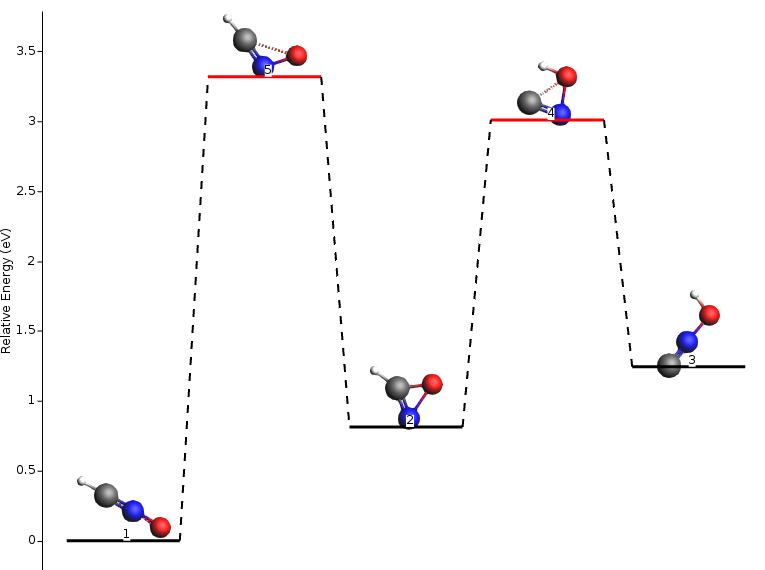
This example performs an Energy Landscape Refinement calculation at the DFTB level of theory on the energy landscape loaded from the previous calculation’s directory results (previous.results). It also loads the coordinates of an additional local minimum (state3) and one transition state (state4) from the input file using the System blocks. The latter transition state is linked to the product state3 (defined in the same input file) and the reactant state with id=2 from the loaded energy landscape (see image above). The output text lines and the graphical representation of the obtained energy landscape are shown below. Notice that the states have been rearranged according to energy.

   Id        Energy(a.u.)         RE(eV)   RE(kcal/mol)    Counts    Crit. point
--------------------------------------------------------------------------------
        -10.424825        0.00000         0.0000         1            Min
        -10.394956        0.81277        18.7428         1            Min
        -10.379113        1.24388        28.6845         1            Min
        -10.314160        3.01134        69.4432         1             TS 2<-->3
        -10.302822        3.31986        76.5577         1             TS 1<-->2

Note

If you want to combine this feature of creating and/or extending an energy landscape with any other job (PESExploration%Job) other than LandscapeRefinement. Don’t forget to include a System block with no header (or label) to define the main chemical system.

Optimizer¶

Geometry optimizations are performed for most PES Explorations job types. In the PESExploration%Optimizer block you may configure some of the parameters for these geometry optimizations:

PESExploration
   Optimizer
      ConvergedForce float
      MaxIterations integer
      Method [CG | QM | LBFGS | FIRE | SD]
   End
End

PESExploration

Optimizer

Type: Block
Description: Configures the details of the geometry optimizers used by the PES explorers.

ConvergedForce

Type: Float
Default value: 0.005
Unit: eV/Angstrom
Description: Convergence threshold for nuclear gradients.

MaxIterations

Type: Integer
Default value: 400
Description: Maximum number of iterations allowed for optimizations.

Method

Type: Multiple Choice
Default value: CG
Options: [CG, QM, LBFGS, FIRE, SD]
Description: Select the method for geometry optimizations.

Binding Sites¶

Binding sites can be determined from an Energy Landscape.

When computing binding sites you will first need to define a reference region, which typically will be a surface or a cluster (regions can be specified in the system input block, or via the “Model → Regions” panel in AMSinput). AMS will then go though all the local minima of Energy Landscape and mark as ‘binding sites’ the positions where an atom of an adsorbed molecule is neighboring atoms in the reference region.

For instance, in Example: PES Exploration, Binding Sites for O on Pt 111, the platinum surface is the reference region, while the oxygen atom is the adsorbate. In the picture below, you can see the oxygen binding sites on the platinum 111 surface (the two different types of binding sites are marked by a blue square and a red triangle respectively).

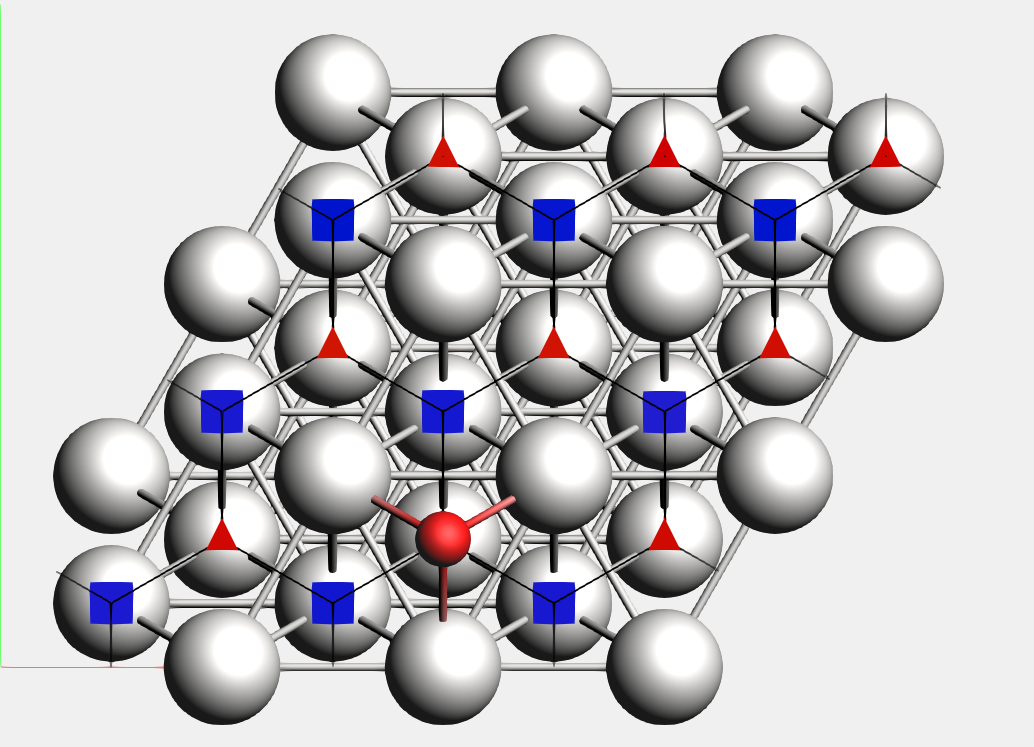
Lines connecting the the binding sites will be drawn if 1) there is a transition state connecting two local minima associated to these binding-sites (notice that may there are multiple local minima associated with the same binding site), and 2) there is at least an atom (from the adsorbate region) that changes its position from the first binding site to the second one mediated by the same transition state described above. In this process, AMS will align as much as possible all local minima and transition states to the input’s file structure but ignoring the atoms in the region adsorbate trying to establish a common reference frame (see also the StatesAlignment input block below).

See also

Binding sites are labeled according to the number of neighbors they have on each of their coordination shells. It has the format N<int><int>.... For example, the label N334 denotes three neighbors in the first shell, three in the second, and four in the third. The parameter PESExploration%BindingSites%MaxCoordinationShellsForLabels or the largest shell contained in the unit cell, determines the maximum number of coordination shells to consider. For labeling purposes, the center of the binding site is taken to be 1.5 Å from the center of the atoms in the first shell in the direction of the adsorbed atom position. PESExploration%BindingSites%DistanceDifference is an important parameter to remember. It is critical because it specifies the tolerance for determining whether or not two atoms are in the same coordination shell based on their distances from the binding site.

The figure below depicts the four types of binding sites observed on a Pt(111) surface. There, you can see the AMS label (e.g., N33, N34, …) as well as the traditional one (e.g., fcc, hcp, …). The distances between the binding site and the highlighted atoms on that coordination shell (or neighborhood) are listed below each geometry. If two numbers are listed, it is because two different distances are involved, but they are considered in the same coordination shell because their difference is less than PESExploration%BindingSites%DistanceDifference.

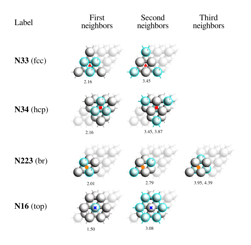
../_images/PESExplorationBindingSitesLabels.png — Fig. 2 Binding sites obtained for a CO molecule adsorbed on a Pt(111) surface using `PESExploration%BindingSites%DistanceDifference = 0.5 Å`.¶

The following is an example of the section in the output file describing the obtained binding sites. In particular, you can find the above details regarding distances involved in calculating their labels.

-------------
Binding Sites
-------------

Number of binding sites:                             4
Number of connections:                               3

Binding sites:

  id   Label   Aver.E(a.u.)  Stdev.E(a.u.)           x         y         z     Parents
   1     N34      -3.773094       0.000000     3.59065   2.09219   3.88471     1(1)
   2     N33      -3.772967       0.000000     4.93783   2.86841   3.88471     2(1)
   3    N223      -3.746180       0.000000     4.25120   2.47351   3.88462     3(1)
   4     N16      -3.683784       0.000000     3.60490   3.59820   3.88382     6(1)

Labels details:

   Label            Center example(A)     Radius(A)
     N33         4.94    2.87    3.88     2.16 - 2.66
                                          3.45 - 3.95
     N34         3.59    2.09    3.88     2.16 - 2.66
                                          3.45 - 3.95
    N223         4.25    2.47    3.88     2.02 - 2.52
                                          2.76 - 3.26
                                          3.86 - 4.36
     N16         3.60    3.60    3.88     1.50 - 2.00
                                          3.04 - 3.54

Input options¶

There are two distinct ways of triggering the computation of binding sites. You can either:

compute the binding sites at the end of a Process Search, Basin Hopping or Landscape Refinement calculation by setting the PESExploration%BindingSites%Calculate option to yes:

PESExploration
  Job [ProcessSearch | BasinHopping | LandscapeRefinement]

  BindingSites
    Calculate Yes
  End

  StatesAlignment
    ReferenceRegion reference_region_name
  End
End

or

compute the binding sites by setting the PESExploration%Job to BindingSites and load a previously computed Energy Landscape (see Example: PES Exploration, Binding Sites for O on Pt 111):

PESExploration
  Job BindingSites

  LoadEnergyLandscape
    Path path/to/previous/calculation/ams.results
  End

  StatesAlignment
    ReferenceRegion reference_region_name
  End
End

The following input options are related to the calculation of binding sites:

PESExploration
   BindingSites
      Calculate Yes/No
      DistanceDifference float
      MaxCoordinationShellsForLabels integer
      NeighborCutoff float
      ReferenceRegion string
   End
End

PESExploration

BindingSites

Type: Block
Description: Options related to the calculation of binding sites.

Calculate

Type: Bool
Default value: No
Description: Calculate binding sites at the end of a job. Not needed for Binding Sites job.

DistanceDifference

Type: Float
Default value: -1.0
Unit: Angstrom
Description: If the distance between two mapped binding-sites is larger than this threshold, the binding-sites are considered different. If not specified, its value will set equal to [PESExploration%StructureComparison%DistanceDifference]

MaxCoordinationShellsForLabels

Type: Integer
Default value: 3
Description: The binding site labels are given based on the coordination numbers of shells in the reference region, using the following format: N<int><int>…, e.g., the label ‘N334’ means 3 atoms in the first coordination shell, 3 in the second one, and 4 in the third one. This parameter controls the maximum number of shells to include.

NeighborCutoff

Type: Float
Default value: -1.0
Unit: Angstrom
Description: Atoms within this distance of each other are considered neighbors for the calculation of the binding sites. If not specified, its value will set equal to [PESExploration%StructureComparison%NeighborCutoff]

ReferenceRegion

Type: String
Default value
Description: Defines the region that is considered as the reference for binding sites detection. Binding sites are projected on this region using the geometry from the reference system. If not specified, its value will set equal to [PESExploration%StatesAlignment%ReferenceRegion]

The following input options are related to the definition of the reference region and alignment thereof:

PESExploration
   StatesAlignment
      DistanceDifference float
      ReferenceRegion string
   End
End

PESExploration

StatesAlignment

Type: Block
Description: Configures details of how the energy landscape configurations are aligned respect to the main chemical system [System].

DistanceDifference

Type: Float
Default value: -1.0
Unit: Angstrom
Description: If the distance between two mapped atoms is larger than this threshold, the configuration is considered not aligned. If not specified, its value will set equal to [PESExploration%StructureComparison%DistanceDifference]

ReferenceRegion

Type: String
Default value
Description: Defines the region that is considered as the reference for alignments. Atoms outside this region are ignored in the alignments.

References¶

1: Samuel T Chill, Matthew Welborn, Rye Terrell, Liang Zhang, Jean-Claude Berthet, Andreas Pedersen, Hannes Jónsson and Graeme Henkelman EON: software for long time simulations of atomic scale systems, Modelling Simul. Mater. Sci. Eng. 22 055002 (2014)
2: David J. Wales and Jonathan P. K. Doye Global Optimization by Basin-Hopping and the Lowest Energy Structures of Lennard-Jones Clusters Containing up to 110 Atoms, J. Phys. Chem. A 1997, 101, 28, 5111–5116
3: G. Henkelman and H. Jónsson, A dimer method for finding saddle points on high dimensional potential surfaces using only first derivatives, J. Chem. Phys. 111, 7010-7022 (1999)
4: A. Heyden, A.T. Bell, and F.J. Keil Efficient methods for finding transition states in chemical reactions: Comparison of improved dimer method and partitioned rational function optimization method, J. Chem. Phys. 123, 224101 (2005)
5: J. Kästner and P. Sherwood Superlinearly converging dimer method for transition state search, J. Chem. Phys. 128, 014106 (2008)
6: R. Malek and N. Mousseau, Dynamics of Lennard-Jones clusters: A characterization of the activation-relaxation technique, Phys. Rev. E 62, 7723 (2000)

Automated PES Exploration¶

Overview¶

Job selection and main options¶

Results: the “Energy Landscape”¶

Results on the text output¶

Continue a PES exploration from a previous calculation¶

Troubleshooting¶

Structure comparison¶

Process Search job¶

Overview¶

Input options¶

Saddle Search job¶

Overview¶

Input options¶

Basin Hopping job¶

Overview¶

Input options¶

Fragmented states¶

Landscape Refinement¶

Creating and/or Extending an Energy Landscape from the Input File¶

Optimizer¶

Binding Sites¶

Input options¶

References¶