Cluster Growth: Cobalt Clusters

Here we show a biased structure search strategy for investigating the structural evolution and growth pattern of single-atom clusters. The strategy consists of adding one atom to the lowest energy structures of the n-atoms (frozen) and get the binding site with the largest binding energy, which is a good approximation to the (n+1)-cluster global minimum structure.

The strategy is illustrated using the Co.ff ReaxFF force field for the growth mechanism Co₈+Co–>Co₉.

The tutorial is divided into two parts: In the first part, we obtain the global minimum for the Co₈ cluster by using the Basin Hopping subtask. In the second part, we fix the coordinates of the Co₈ global minimum, add a Co atom and use the Process Search subtask to obtain all reaction mechanisms involving it, and with them, the corresponding binding sites. The structure associated with the highest binding energy is the best approximation to the Co₉ global minimum structure, and the binding-sites lattice will give us insights into the growth mechanism behind it. The gradual population of the binding sites shows the structural evolution and the growth pattern of these kinds of clusters.

Hereafter, we will use the PES exploration task in the AMS driver with the ReaxFF engine. Configure this by following the steps below:

1. Start AMSinput (SCM → New Input).

2. In AMSinput, select the ReaxFF panel: → .

3. Select the Task → PES Exploration.

4. Select Periodicity → None.

5. Select the Force field → Co.ff.

Global Optimization of Co₈

We need an initial guess for the structure of the Co₈ cluster. Thus, create a random structure composed of 8 atoms of Co by using the drawing tools of AMSinput. Avoid a planar configuration for the cluster’s atoms; to do so, take some atoms out of that plane individually if needed. The difficulty is that planar configurations usually converge to a transition state during optimization instead of a local minimum. Then, use the Pre-optimize button on the main panel to get the closest local minimum, make sure to pre-optimize the full structure. Make sure that you have a non-flat structure with none of the atoms collapsed. Otherwise try rebuilding an 8-atom cluster again. This step is summarized in the following Figure:

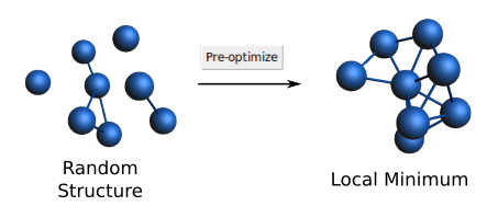
The initial structure is not important, but more iterations may be needed to get the same results. For this tutorial, we suggest starting with the same local minimum to improve reproducibility.

1. Delete your current structure by clicking Select → Select all and pressing the Delete key.

2. Copy & paste the coordinates below into AMSinput.

3. Press the Pre-optimize button again.

Co      -0.57747929       3.09962106      -1.40010667
Co      -1.94268805       1.60982864      -0.21835532
Co       0.68130178      -0.28713038       1.61855474
Co       0.41911715       1.21862699      -0.30327160
Co       1.35380790       3.40899190      -0.11445733
Co       1.88623229       1.82216225       1.57360827
Co       0.56876970      -1.15098318      -0.59251345
Co       2.52877908       0.02596128       0.06823723

To setup the Basin Hopping calculation, follow these steps:

1. Select Task → PES Exploration.

2. Click on next to the Task to specify the PES Exploration settings.

3. On the PES Exploration page, select Job → Basin Hopping.

4. Set Num expeditions to 10.

5. Set Num explorers to 4.

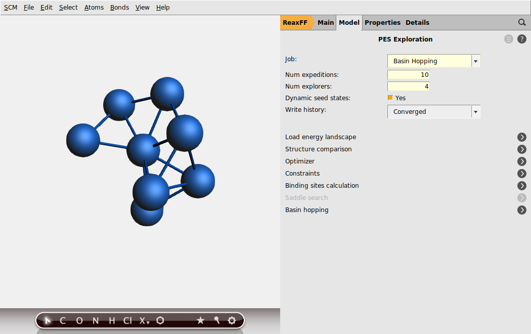
Details on the different settings can be found in the PES exploration page in the AMS driver manual. For the purpose of this tutorial we will leave everything at the default values, except the number of expeditions and the number of explorers per expedition.

We have now finished the setup of the calculation and we are ready to run it:

1. Select File → Save As and give it an appropriate name (e.g. Co8_BH)

2. Select File → Run

3. Wait for the calculation to finish (this should take a few seconds)

We can visualize the explored energy landscape by using AMSmovie:

1. Select SCM → Movie

2. In AMSmovie, make a double click on the Energy axis and change the units to eV. Y Axis → Units: eV then OK.

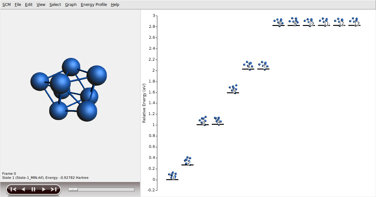
With some luck, the lowest energy state should be at -0.927817 Hartree. If so, we have caught the global minimum successfully! Pass the mouse over the state to verify the exact value of the energy.

Basin Hopping optimization is a global optimization that uses random perturbations to jump basins, and a local search algorithm to optimize each basin. So, results may vary given the stochastic nature of the algorithm or differences in numerical precision. Consider running the example a few times and compare the outcomes.

For the next step, we will use the Co₈ global minimum. So, copy its geometry and paste it into a new AMSinput.

1. Make a right-click on the lowest energy state and select the option Copy Geometry from the popup menu.

2. Start a new AMSinput SCM → New Input.

3. Paste the geometry by using Edit → Paste or just press ctrl+v.

Growth Mechanism Co₈+Co → Co₉

Firstly, we need the geometry of the Co₈ global minimum obtained in the previous section. In case you skipped the previous section, just copy-paste the following coordinates into AMSinput.

Co      -0.03403571       1.12611646      -2.08186475
Co      -1.53717952       1.78357073      -0.30583453
Co       1.68546231      -0.17156299       1.49980432
Co      -0.01541891       1.59507948       1.61007493
Co       0.67964989       2.82625193      -0.46130535
Co       2.34451750       2.13563230       1.20356390
Co      -0.20262505      -0.26260499      -0.06462506
Co       1.99747005       0.71459565      -0.76811757

The new AMSinput window does not know yet that we want to perform PES explorations with the ReaxFF engine. Let us quickly restore the engine settings we have used for the Basin Hopping earlier:

1. In AMSinput, select the ReaxFF panel: → .

2. Select the Task → PES Exploration.

3. Select the Force field → Co.ff.

4. Make sure Periodicity is set to None.

Using the drawing tools of AMSinput, add a new Co atom roughly on the cluster’s surface. Then, use the Pre-optimize button to get the closest local minimum, making sure that only the new atom is selected, and only that selection is optimized; we would like to keep the structure of the Co₈ intact. Again, the initial structure is not important, but more iterations may be needed to get the same results. We suggest starting with the following coordinates to improve reproducibility. But, we invite you to use the first option to compare times and outcomes.

Co      -0.03403571       1.12611646      -2.08186475
Co      -1.53717952       1.78357073      -0.30583453
Co       1.68546231      -0.17156299       1.49980432
Co      -0.01541891       1.59507948       1.61007493
Co       0.67964989       2.82625193      -0.46130535
Co       2.34451749       2.13563230       1.20356390
Co      -0.20262505      -0.26260499      -0.06462506
Co       1.99747005       0.71459565      -0.76811757
Co       3.01465991       2.87039628      -0.97767612

First, we would like to define two regions: 1) adsorbate, corresponding to the added atom, and 2) cluster, corresponding to the Co₈ global minimum. Then, we use the defined cluster region to fix the coordinates of the Co₈.

1. Use the panel bar Model → Regions command

2. Select the added atom

3. Click on the ‘+’ button to add a new region

4. Change the name Region_1 into adsorbate

5. Select the Co₈ atoms (Select → Invert Selection)

6. Click on the ‘+’ button to add a new region

7. Change the name Region_2 into cluster

8. Use the panel bar Model → Geometry Constraints and PES Scan command

9. Make sure at least one atom from the cluster region is selected

10. Click on the ‘+’ cluster (fixed position) button to to fix the coordinates of the Co₈

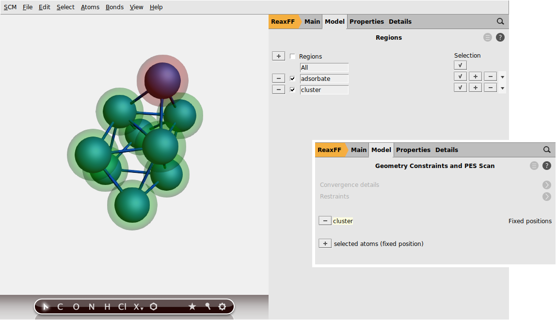
In this step, we are interested in exploring all possible processes in which the added atom may be involved. Here, we will use the Process Search subtask for this aim. To clarify, we refer to processes as paths that connect local minima through saddle points (transition states). The subtask Process Search will start in the proposed local minimum and try to find a nearby saddle point starting from a random displacement of the added atom. If a saddle point is found, it will perform a geometry optimization pushing the atom to the other side of the saddle point to find the new local minimum to which the original state is connected. This process is repeated several times, starting from all the local minima discovered so far.

Once the energy landscape is obtained, we will also ask to calculate the associated binding-sites lattice. Binding sites are defined as the atoms’ position from the adsorbate region which are neighbors of the atoms in the region cluster and associated with a local minimum configuration in the energy landscape. Additionally, two binding sites are considered connected if the following two requirements are met: 1) there is a transition state connecting two local minima associated to these binding sites (notice that there may be multiple local minima associated with the same binding site), and 2) there is at least an atom (from the adsorbate region) that changes its position from the first binding site to the second one mediated by the same transition state described above. In this process, AMS will align as much as possible all local minima and transition states to the input file’s structure but ignoring the atoms in the region adsorbate trying to establish a common reference frame. If the structure of the region cluster changes significantly for different configurations, the binding sites may not be well defined. For this example, we have frozen the Co₈ cluster region, which guarantees that we will not have that issue.

To setup the Process Search calculation, follow these steps:

1. Go to the Model → PES Exploration panel.

2. On the PES Exploration page, select Job → Process Search.

4. Set Num expeditions to 100.

5. Set Num explorers to 4.

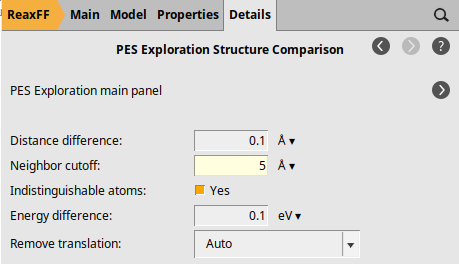
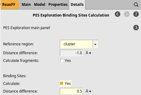
6. Click on next to the Structure Comparison

7. On the PES Exploration Structure Comparison page, set Neighbors cutoff to 5.0 Å

8. Go to Details → PES Exploration… → PES Exploration Binding sites calculation

9. On the PES Exploration Binding sites calculation page, select cluster as the Reference region

10. E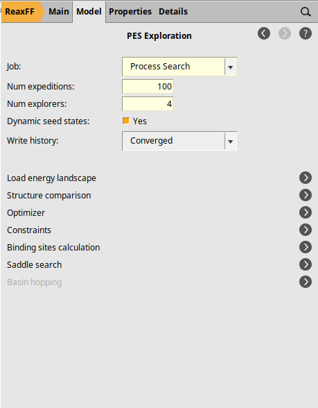nable the calculation of the binding sites by selecting the option Calculate under the Binding Sites section.

11. Set Distance difference to 0.5 Å.

We have now finished the setup of the calculation and we are ready to run it:

1. Select File → Save As and give it an appropriate name (e.g. Co8+Co_PS)

2. Select File → Run

3. Wait for the calculation to finish (this should take a few minutes). Click Yes when asked to load the binding sites in AMSinput.

In the AMSinput, we will see the binding-sites lattice superimposed to the cluster’s initial geometry:

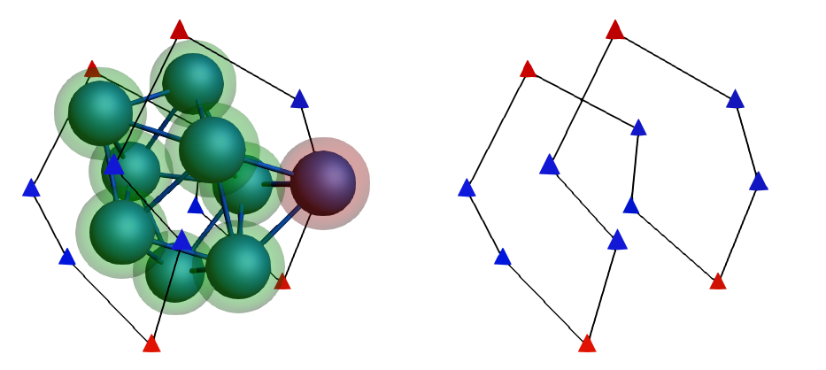
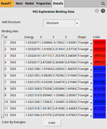
Notice that the added atom is located over one of the binding sites. The symbols used to represent the binding sites are related to the number of atom neighbors (within a 5 Å of distance, see above Neighbors cutoff option) and the colors with the average energy of the contributing states. In our case, because there is only one type of neighborhood, there is only one symbol: triangles. These binding sites have three neighbors in the first coordination shell and three neighbors in the second. Because of this, the labels are N33. Regarding their color, we have two groups: 1) Red for the most stable adsorption-sites with the energy of around -1.0333 Hartree, and 2) Blue for the rest of the binding sites with the energy of -1.0321 Hartree. These details can be seen from the panel Details → PES Exploration Binding Sites:

We can visualize the explored energy landscape by using AMSmovie:

1. In the AMSJobs window, select the job and click SCM → Movie

2. In AMSmovie, double-click the Energy axis and change the units, e.g., to eV. Y Axis → Units: eV then OK.

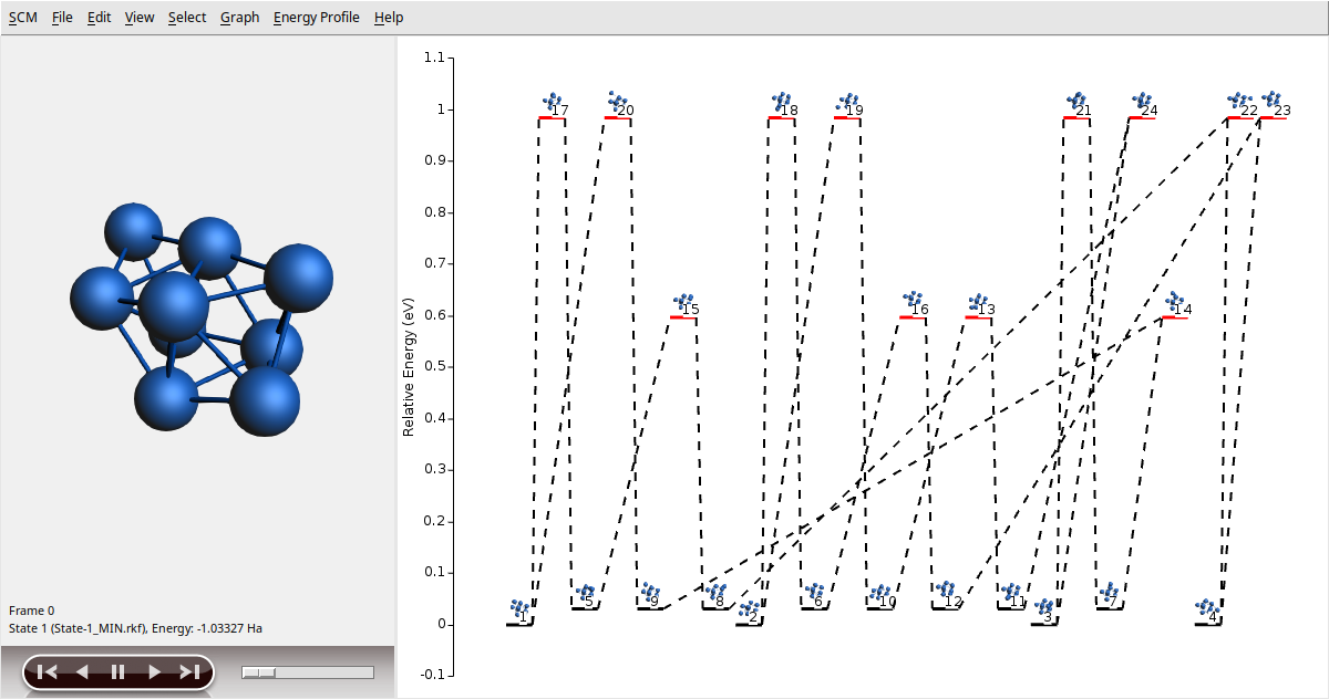
You should get a graphical representation of the states discovered during the searching in the right panel. Minima are shown with a black level, while transition states are shown using a red level. You can move around the different states by clicking on them. The selected state is shown on the left panel to appreciate details.

As a final comment, due to the stochastic nature of the algorithm and/or differences in numerical precision, you can get different results for the energy landscape exploration. In our example, particularly, we have chosen 100 for Num expeditions to guarantee that you can get the full set of critical points; 12 local minima and 12 transition states.

Note

You can see the vibrational spectrum of any state by using right-click on it and then selecting Open in module → Spectra in the popup window. For the present calculation, only the frequencies of the modes related to the unconstrained atoms are available.

Note

You can remove any state by using right-click on it and then selecting Delete level in the popup window.

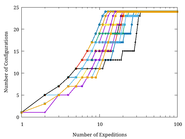
In the Figure below, we show the number of configurations obtained by 20 different runs as the number of expeditions increase. Notice that at least 100 expeditions are required to guarantee you get the 24 configurations.