Nudged Elastic Band (NEB)
In this tutorial we will use the climbing-image Nudged Elastic Band method (NEB) to identify the minimum energy path of:
Transition state of a chemical reaction
In this first example, we will find the minimum energy reaction path and transition state of the following reaction:
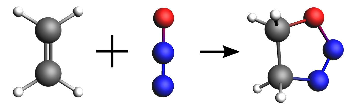
We will be using the DFTB engine with the GFN1-xTB model. This is a computationally fast method (which is convenient for the purposes of a tutorial) but it is not very accurate in predicting reaction energies. For better accuracy, using the DFT engine ADF (or BAND) is recommended.
Setting up and running the calculation
You can set up and run the calculations for this tutorial using either the Graphical User Interface (GUI), the python library PLAMS or a bash script.
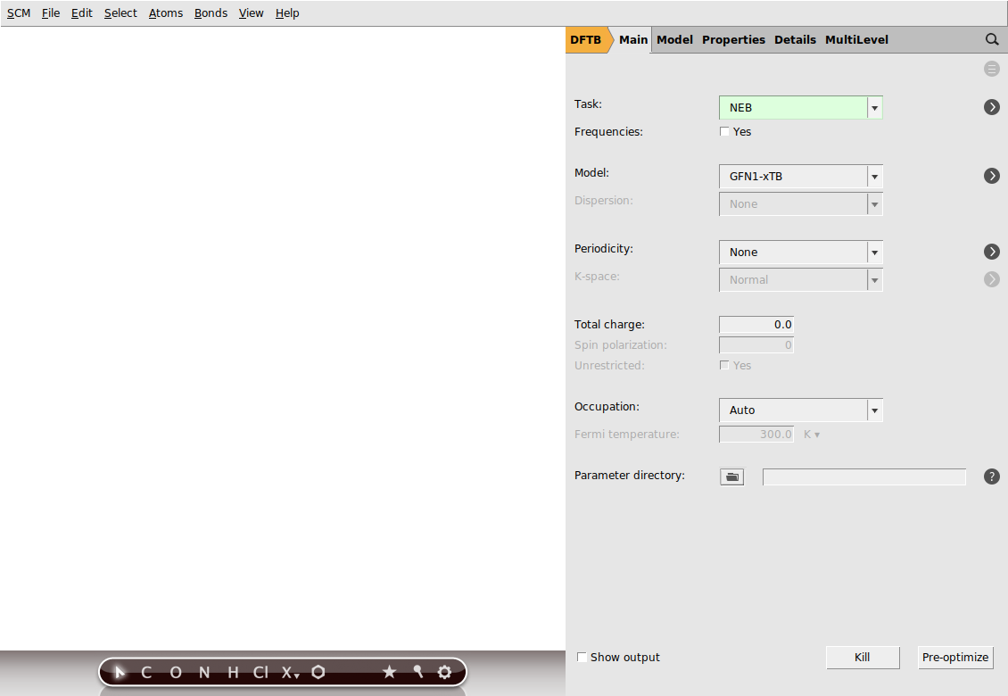
This will open a new AMSinput window.
 →
→ 
We will use the GFN1-xTB model, which is the default model as of the AMS2020 release. Your AMSinput window should look like this:
When setting up an NEB calculation we need to specify two systems: the initial and final states of the reaction. The NEB algorithm will then generate a set of images by interpolating between the initial and final systems. This will be the initial approximation of the reaction path, which will be optimized during the NEB calculation.
NEB_initial.xyz and NEB_final.xyzYou can easily switch between molecule tabs using the arrows at the bottom of the molecule drawing area. Here, you’ll also see the molecule names, such as C2H4N2O for the first molecule and NEB_final for the second. Note that the GUI has the following naming convention:
Main System: The first molecule is considered the main system, and is often automatically assigned its chemical formula as the name.
Additional Molecules: For any additional molecules, the GUI uses by default the name from their original XYZ files.
Important
In NEB calculations, the order of the atoms in the initial and final system should be the same (if you provide an intermediate system, you should use a consistent atom-ordering for that too). The order of the atoms should be consistent because the images-interpolation algorithm maps the n-th atom of the initial system to the n-th atom of the final system.
You can see the indices of the atoms by clicking in the menu bar on Properties → Atom Info → Name → Show. It is possible to change the order of the atoms in the Coordinates panel (in the panel bar: Model → Coordinates) using the Move atom(s) option.
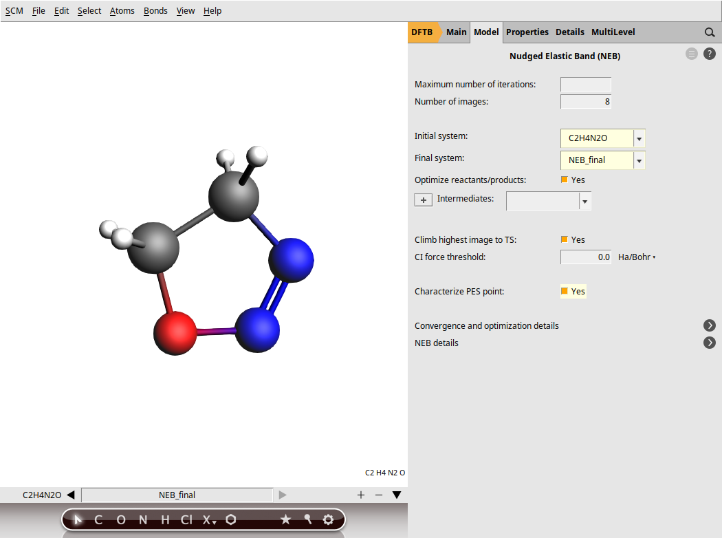
Now, go to the NEB details panel where we will set up the NEB calculation:
 next to Task → NEB to go to the NEB details panel
Your AMSinput window should look like this:
Tip
From most AMSinput panels you can jump to the relevant section of the user manual by clicking on  , which is located in the top-right corner of the panel.
We are now ready to run the calculation:
In the logfile you can monitor the progress of your NEB calculation:
A NEB calculation consists of several steps, which are automatically executed one after the other:
first, the two end points (the initial and final molecules) are optimized (in the logfile, look for
Optimizing initial stateandOptimizing final state)then the NEB reaction path will be optimized (in the logfile, look for
NEB Path Optimization). During the reaction path optimization, the highest-energy image on the path will climb to the transition statefinally, a single point calculation for the TS is performed (in the logfile:
Final calculation for highest-energy image). If the option Characterize PES point is on, then the lowest-lying normal modes will be calculated in order to validate the TS (the TS should have exactly one imaginary frequency). Some information on the reaction path is printed at the end of the logfile:NEB found a transition state! TS barrier height from the left 0.02576078 Hartree 16.165 kcal/mol 67.635 kJ/mol TS barrier height from the right 0.08632064 Hartree 54.167 kcal/mol 226.635 kJ/mol
The following bash script performs an NEB calculation using the AMS driver and the DFTB engine. The input options for the AMS driver described in the AMS driver manual, while the DFTB manual describes the input options for the DFTB Engine block.
#!/bin/sh

"$AMSBIN/ams" << eor

Task NEB

Properties
    PESPointCharacter Yes
End

# The initial system (no header)
System
    Atoms
        N  1.88630912 -0.34204867 -1.59424245
        N  1.14203025 -1.15084766 -1.95458206
        O  0.07639739 -1.27682918 -1.40578886
        C  0.74766633  1.24132374  1.29097263
        C -0.52735637  0.87051548  1.20080269
        H  1.08791192  2.15092371  0.80682956
        H -1.23438622  1.47569873  0.64278673
        H -0.86675778 -0.04061999  1.68265930
        H  1.45534611  0.63457332  1.84647164
    End
End

# The final system should be called 'final'
System final
    Atoms
        N  1.44280525  0.39326405  0.02115802
        N  0.56588608 -0.32983790 -0.53167497
        O -0.68785300 -0.26603404 -0.00725496
        C  0.86550207  1.12517445  1.10513146
        C -0.57889386  0.65549932  1.05974328
        H  0.94852175  2.21696742  0.91684905
        H -1.26384434  1.51200042  0.88137995
        H -0.85746564  0.15513847  2.01191277
        H  1.35845740  0.84559176  2.06071421
    End
End

Engine DFTB
    Model GFN1-xTB
EndEngine
eor
Important
In NEB calculations, the order of the atoms in the initial and final system should be the same (if you provide an intermediate system, you should use a consistent atom-ordering for that too). The order of the atoms should be consistent because the images-interpolation algorithm maps the n-th atom of the initial system to the n-th atom of the final system.
To run the calculation:
NEB.runchmod +x NEB.run./NEB.run > outSee the NEB scripting example.
To improve the initial approximation of the reaction path in an NEB calculation, you can (optionally) provide an intermediate system.
Another important NEB option is the number of images. In case of problematic NEB path optimization convergence, using more images might help (note that the computation time increases with the number of images used).
You can read more about the various NEB options in the AMS manual.
Results of the calculation
Now, let’s visualize the reaction path computed by NEB:
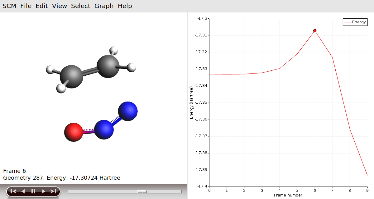
In AMSmovie, you can click on play (or drag the slide-bar) so see the reaction happening. On right-hand side, the energy and gradients of the images in the NEB reaction path are plotted.
The transition state is characterized by having one imaginary frequency. Let’s visualize the normal modes of the transition state geometry with AMSspectra:
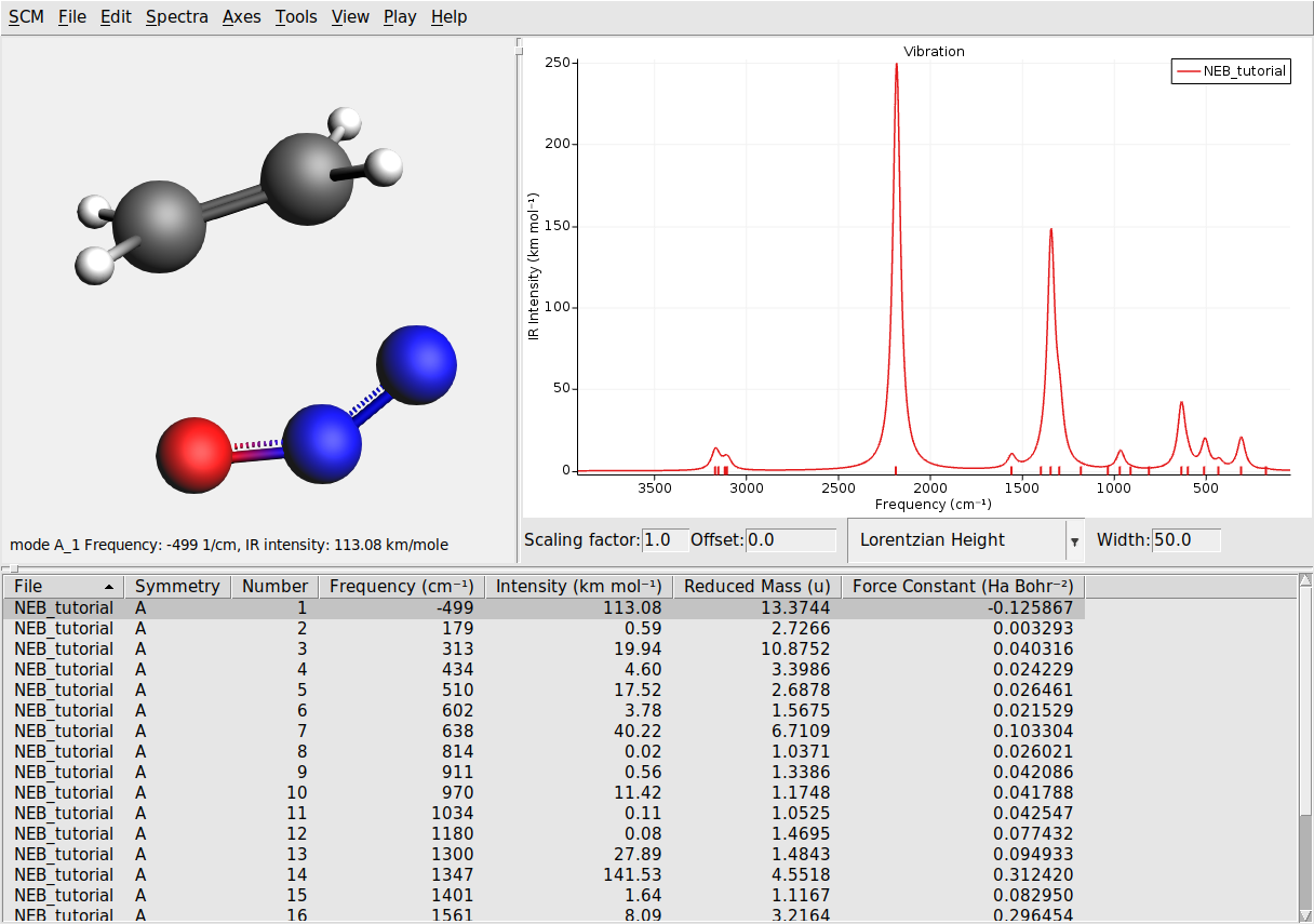
Here you will see the computed normal modes for the TS geometry. Notice that there is one negative frequency (imaginary frequency are shown as negative numbers).
The corresponding normal mode will be displayed in the molecule-visualization area. This normal mode gives you an idea of how the atoms are moving as they cross the transition state.
In the folder where you executed your script you will find a file out, which contains the text-output of the calculation, and a folder called ams.results containing binary results of the calculation.
At the end of the output file out you will find a section summarizing the results of the NEB calculation:
NEB found a transition state!


------------------------------------------------------------
TS barrier height from the left           0.02581511 Hartree
                                         16.199 kcal/mol
                                         67.778 kJ/mol
TS barrier height from the right          0.08637041 Hartree
                                         54.198 kcal/mol
                                        226.765 kJ/mol
Reaction energy                          -0.06055530 Hartree
                                        -37.999 kcal/mol
                                       -158.988 kJ/mol
------------------------------------------------------------
        Transition state geometry

--------
Geometry
--------

Atoms
Index Symbol   x (angstrom)   y (angstrom)   z (angstrom)
   1      N     1.76794468     0.02199401    -0.76530642
   2      N     0.86568320    -0.56021023    -1.14090273
   3      O    -0.28459962    -0.76023024    -0.92163051
   4      C     0.89983351     0.97770099     0.84893165
   5      C    -0.38912967     0.55813520     0.80607959
   6      H     1.18303105     1.94163319     0.44757192
   7      H    -1.15509240     1.14579400     0.31965225
   8      H    -0.73127815    -0.27639812     1.40152984
   9      H     1.61076814     0.51427067     1.51998360
The folder ams.results contains:
a text file called
ams.logcontaining a very concise summary of the calculation’s progress during the run.the main binary results file
ams.rkf, containing the reaction path computed in the NEB calculation.the engine results file
NEB_TS_final.rkfcorresponding a single point calculation at the transition state geometry. It contains, among other properties, the normal modes.
You can explore the content of the rkf binary results files using the kfbrowser utility.
$AMSBIN/kfbrowser ams.results/NEB_TS_final.rkfThe binary results of the calculation can also be visualized with the GUI modules:
$AMSBIN/amsmovie ams.results/ams.rkf$AMSBIN/amsspectra ams.results/NEB_TS_final.rkfIonic diffusion in a solid
In this second example, we will determine the minimum energy path and the activation energy of Li diffusion in a typical cathode materials LiTiS2.
We will use the ML potential engine with the M3GNet universal machine learning potential. Although M3GNet was trained to reproduce ground state structures of the Materials Project database, it can also be accurate to describe transition states, as we will demonstrate in this tutorial. This tutorial can be reproduced with the periodic DFT engine BAND.
Important
First, make sure to install the M3GNet package inside AMS as described in the M3GNet tutorial.
Note
When using M3GNet, you can include dispersion via an “engine addon” option. In the following, D3 dispersion will be included throughout.
Layer LiTiS2 cathode material
In some Li-based cathode materials, the diffusion of Li ions is tightly connected to the content of Li in the materials. We would like to demonstrate this by computing
the diffusion barrier of Li in LiTiS2 with 1 Li vacancy, and
the diffusion barrier of Li in LiTiS2 with 2 Li vacancies.
In LiTiS2, the lithium ions are octahedrally coordinated between the S−Ti−S sandwich layers.
Li diffusion in LiTiS2 with 1 vacancy
To perform the NEB calculation we will use the graphical user interface. Either
build the systems manually (next step), or
import them directly (skip to the next section)
Build LiTiS2 initial and final structures with 1 vacancy
We will start with a supercell of crystalline LiTiS2, constructed from the optimized lattice parameters, and then introduce a vacancy.
Import the pristine system
Now, either
download
LiTiS2_supercell_pristine.inand import it (File → Import coordinates…), orcopy-paste the below coordinates into AMSinput.
Reveal copy-pastable coordinates
System
    Atoms
        Li 1.71915 2.9776551458 6.174905
        Ti 1.71915 2.9776551458 3.0874525
        S 1.71915 4.9627585764 4.5513282748
        S 3.4383 3.9702068611 7.7984817252
        Li 3.4383 5.9553102917 0.0
        Ti 3.4383 5.9553102917 9.2623575
        S 3.4383 7.9404137222 10.7262332748
        S 5.15745 6.947862007 1.6235767252
        Li 3.4383 5.9553102917 6.174905
        Ti 3.4383 5.9553102917 3.0874525
        S 3.4383 7.9404137222 4.5513282748
        S 5.15745 6.947862007 7.7984817252
        Li 6.8766 0.0 0.0
        Ti 6.8766 0.0 9.2623575
        S 6.8766 1.9851034305 10.7262332748
        S 8.595750000000001 0.9925517153 1.6235767252
        Li 6.8766 0.0 6.174905
        Ti 6.8766 0.0 3.0874525
        S 6.8766 1.9851034305 4.5513282748
        S 8.595750000000001 0.9925517153 7.7984817252
        Li 5.15745 2.9776551458 0.0
        Ti 5.15745 2.9776551458 9.2623575
        S 5.15745 4.9627585764 10.7262332748
        S 6.8766 3.9702068611 1.6235767252
        Li 5.15745 2.9776551458 6.174905
        Ti 5.15745 2.9776551458 3.0874525
        S 5.15745 4.9627585764 4.5513282748
        S 6.8766 3.9702068611 7.7984817252
        Li -3.4383 5.9553102917 0.0
        Ti -3.4383 5.9553102917 9.2623575
        S -3.4383 7.9404137222 10.7262332748
        S -1.71915 6.947862007 1.6235767252
        Li -3.4383 5.9553102917 6.174905
        Ti -3.4383 5.9553102917 3.0874525
        S -3.4383 7.9404137222 4.5513282748
        S -1.71915 6.947862007 7.7984817252
        Li 0.0 0.0 0.0
        Ti 0.0 0.0 9.2623575
        S 0.0 1.9851034305 10.7262332748
        S 1.71915 0.9925517153 1.6235767252
        Li 0.0 0.0 6.174905
        Ti 0.0 0.0 3.0874525
        S 0.0 1.9851034305 4.5513282748
        S 1.71915 0.9925517153 7.7984817252
        Li -1.71915 2.9776551458 0.0
        Ti -1.71915 2.9776551458 9.2623575
        S -1.71915 4.9627585764 10.7262332748
        S 0.0 3.9702068611 1.6235767252
        Li -1.71915 2.9776551458 6.174905
        Ti -1.71915 2.9776551458 3.0874525
        S -1.71915 4.9627585764 4.5513282748
        S 0.0 3.9702068611 7.7984817252
        Li 0.0 5.9553102917 0.0
        Ti 0.0 5.9553102917 9.2623575
        S 0.0 7.9404137222 10.7262332748
        S 1.71915 6.947862007 1.6235767252
        Li 0.0 5.9553102917 6.174905
        Ti 0.0 5.9553102917 3.0874525
        S 0.0 7.9404137222 4.5513282748
        S 1.71915 6.947862007 7.7984817252
        Li 3.4383 0.0 0.0
        Ti 3.4383 0.0 9.2623575
        S 3.4383 1.9851034305 10.7262332748
        S 5.15745 0.9925517153 1.6235767252
        Li 3.4383 0.0 6.174905
        Ti 3.4383 0.0 3.0874525
        S 3.4383 1.9851034305 4.5513282748
        S 5.15745 0.9925517153 7.7984817252
        Li 1.71915 2.9776551458 0.0
        Ti 1.71915 2.9776551458 9.2623575
        S 1.71915 4.9627585764 10.7262332748
        S 3.4383 3.9702068611 1.6235767252
    End
    Lattice
        10.3149 0.0 0.0
        -5.15745 8.9329654375 0.0
        0.0 0.0 12.34981
    End
End
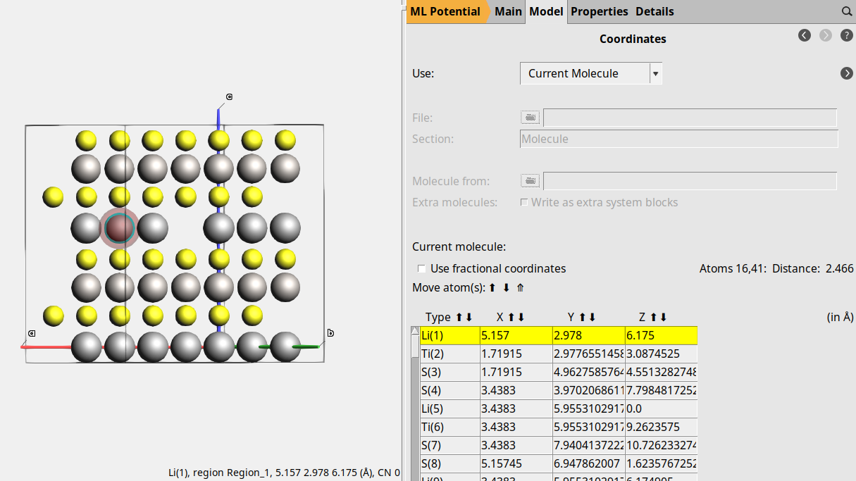
Create the “initial” system for NEB with a Li vacancy
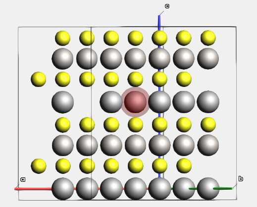
Orient the crystal along the x-axis (Ctrl+1), then rotate the view slightly the molecule for a better view of the middle Li atom in the top layer (index 25).
5.157 2.978 6.175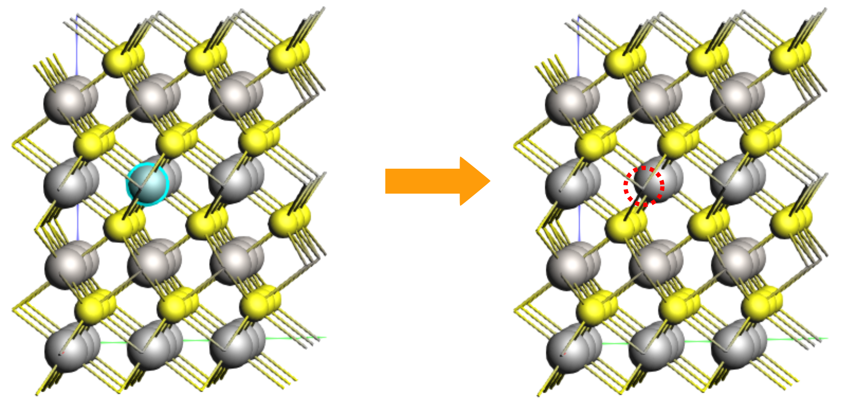
The Li atom that will diffuse has index 1. Let’s highlight it with a region for better visibility. Regions can be used to affect the calculation, but here we just use it to better see the diffusing atom.
This will highlight atom 1 with a colored orb around it.
Now export this structure to a .in file, so that we do not accidentally lose it:
LiTiS2_vacancy_initial.inCreate the “final” system for NEB with a Li vacancy
NEB calculations have both a starting point (initial system) and an end point (final system).
We will create the final system by changing the coordinates of atom 1 to the coordinates of the atom
that was removed.
You can either do this
manually by first selecting atom 1 and then right-click-dragging the atom into the approximate position of the previous vacancy, or
just set the coordinates directly:
In the panel bar, go to Model → CoordinatesChange the coordinates of the first atom to5.157 2.978 6.175(the values for the atom you removed earlier)File → Export coordinates → .inUse the file nameLiTiS2_vacancy_final.in
Set up the NEB calculation
Import the initial and final systems
Note
By default, the NEB task will optimize both the initial and final points before interpolating between them.
Make sure that the initial and final structures are close to their respective local minima!
Best practice is to explicitly optimize them and verify that the structures look good before running the NEB.
When you perform NEB in a crystal it is recommended to keep the cell dimension between the initial and final states.
Create a new clean input:
Now, either
File → Import Coordinates →
LiTiS2_vacancy_initial.in(download or use your own), orReveal copy-pasteable coordinates (LiTiS2_vacancy_initial.in)
System
    Atoms
        Li 1.71915 2.9776551458 6.174905 region=Region_1
        Ti 1.71915 2.9776551458 3.0874525
        S 1.71915 4.9627585764 4.5513282748
        S 3.4383 3.9702068611 7.7984817252
        Li 3.4383 5.9553102917 0.0
        Ti 3.4383 5.9553102917 9.2623575
        S 3.4383 7.9404137222 10.7262332748
        S 5.15745 6.947862007 1.6235767252
        Li 3.4383 5.9553102917 6.174905
        Ti 3.4383 5.9553102917 3.0874525
        S 3.4383 7.9404137222 4.5513282748
        S 5.15745 6.947862007 7.7984817252
        Li 6.8766 0.0 0.0
        Ti 6.8766 0.0 9.2623575
        S 6.8766 1.9851034305 10.7262332748
        S 8.595750000000001 0.9925517153 1.6235767252
        Li 6.8766 0.0 6.174905
        Ti 6.8766 0.0 3.0874525
        S 6.8766 1.9851034305 4.5513282748
        S 8.595750000000001 0.9925517153 7.7984817252
        Li 5.15745 2.9776551458 0.0
        Ti 5.15745 2.9776551458 9.2623575
        S 5.15745 4.9627585764 10.7262332748
        S 6.8766 3.9702068611 1.6235767252
        Ti 5.15745 2.9776551458 3.0874525
        S 5.15745 4.9627585764 4.5513282748
        S 6.8766 3.9702068611 7.7984817252
        Li -3.4383 5.9553102917 0.0
        Ti -3.4383 5.9553102917 9.2623575
        S -3.4383 7.9404137222 10.7262332748
        S -1.71915 6.947862007 1.6235767252
        Li -3.4383 5.9553102917 6.174905
        Ti -3.4383 5.9553102917 3.0874525
        S -3.4383 7.9404137222 4.5513282748
        S -1.71915 6.947862007 7.7984817252
        Li 0.0 0.0 0.0
        Ti 0.0 0.0 9.2623575
        S 0.0 1.9851034305 10.7262332748
        S 1.71915 0.9925517153 1.6235767252
        Li 0.0 0.0 6.174905
        Ti 0.0 0.0 3.0874525
        S 0.0 1.9851034305 4.5513282748
        S 1.71915 0.9925517153 7.7984817252
        Li -1.71915 2.9776551458 0.0
        Ti -1.71915 2.9776551458 9.2623575
        S -1.71915 4.9627585764 10.7262332748
        S 0.0 3.9702068611 1.6235767252
        Li -1.71915 2.9776551458 6.174905
        Ti -1.71915 2.9776551458 3.0874525
        S -1.71915 4.9627585764 4.5513282748
        S 0.0 3.9702068611 7.7984817252
        Li 0.0 5.9553102917 0.0
        Ti 0.0 5.9553102917 9.2623575
        S 0.0 7.9404137222 10.7262332748
        S 1.71915 6.947862007 1.6235767252
        Li 0.0 5.9553102917 6.174905
        Ti 0.0 5.9553102917 3.0874525
        S 0.0 7.9404137222 4.5513282748
        S 1.71915 6.947862007 7.7984817252
        Li 3.4383 0.0 0.0
        Ti 3.4383 0.0 9.2623575
        S 3.4383 1.9851034305 10.7262332748
        S 5.15745 0.9925517153 1.6235767252
        Li 3.4383 0.0 6.174905
        Ti 3.4383 0.0 3.0874525
        S 3.4383 1.9851034305 4.5513282748
        S 5.15745 0.9925517153 7.7984817252
        Li 1.71915 2.9776551458 0.0
        Ti 1.71915 2.9776551458 9.2623575
        S 1.71915 4.9627585764 10.7262332748
        S 3.4383 3.9702068611 1.6235767252
    End
    Lattice
        10.3149 0.0 0.0
        -5.15745 8.9329654375 0.0
        0.0 0.0 12.34981
    End
End
Create a new “molecule” in AMSinput for the final state:
Now, either
File → Import Coordinates →
LiTiS2_vacancy_final.in(download or use your own), orReveal copy-pasteable coordinates (LiTiS2_vacancy_final.in)
System
    Atoms
        Li 5.157 2.9776551458 6.174905 region=Region_1
        Ti 1.71915 2.9776551458 3.0874525
        S 1.71915 4.9627585764 4.5513282748
        S 3.4383 3.9702068611 7.7984817252
        Li 3.4383 5.9553102917 0.0
        Ti 3.4383 5.9553102917 9.2623575
        S 3.4383 7.9404137222 10.7262332748
        S 5.15745 6.947862007 1.6235767252
        Li 3.4383 5.9553102917 6.174905
        Ti 3.4383 5.9553102917 3.0874525
        S 3.4383 7.9404137222 4.5513282748
        S 5.15745 6.947862007 7.7984817252
        Li 6.8766 0.0 0.0
        Ti 6.8766 0.0 9.2623575
        S 6.8766 1.9851034305 10.7262332748
        S 8.595750000000001 0.9925517149999999 1.6235767252
        Li 6.8766 0.0 6.174905
        Ti 6.8766 0.0 3.0874525
        S 6.8766 1.9851034305 4.5513282748
        S 8.595750000000001 0.9925517149999999 7.7984817252
        Li 5.15745 2.9776551458 0.0
        Ti 5.15745 2.9776551458 9.2623575
        S 5.15745 4.9627585764 10.7262332748
        S 6.8766 3.9702068611 1.6235767252
        Ti 5.15745 2.9776551458 3.0874525
        S 5.15745 4.9627585764 4.5513282748
        S 6.8766 3.9702068611 7.7984817252
        Li -3.4383 5.9553102917 0.0
        Ti -3.4383 5.9553102917 9.2623575
        S -3.4383 7.9404137222 10.7262332748
        S -1.71915 6.947862007 1.6235767252
        Li -3.4383 5.9553102917 6.174905
        Ti -3.4383 5.9553102917 3.0874525
        S -3.4383 7.9404137222 4.5513282748
        S -1.71915 6.947862007 7.7984817252
        Li 0.0 0.0 0.0
        Ti 0.0 0.0 9.2623575
        S 0.0 1.9851034305 10.7262332748
        S 1.71915 0.9925517149999999 1.6235767252
        Li 0.0 0.0 6.174905
        Ti 0.0 0.0 3.0874525
        S 0.0 1.9851034305 4.5513282748
        S 1.71915 0.9925517149999999 7.7984817252
        Li -1.71915 2.9776551458 0.0
        Ti -1.71915 2.9776551458 9.2623575
        S -1.71915 4.9627585764 10.7262332748
        S 0.0 3.9702068611 1.6235767252
        Li -1.71915 2.9776551458 6.174905
        Ti -1.71915 2.9776551458 3.0874525
        S -1.71915 4.9627585764 4.5513282748
        S 0.0 3.9702068611 7.7984817252
        Li 0.0 5.9553102917 0.0
        Ti 0.0 5.9553102917 9.2623575
        S 0.0 7.9404137222 10.7262332748
        S 1.71915 6.947862007 1.6235767252
        Li 0.0 5.9553102917 6.174905
        Ti 0.0 5.9553102917 3.0874525
        S 0.0 7.9404137222 4.5513282748
        S 1.71915 6.947862007 7.7984817252
        Li 3.4383 0.0 0.0
        Ti 3.4383 0.0 9.2623575
        S 3.4383 1.9851034305 10.7262332748
        S 5.15745 0.9925517149999999 1.6235767252
        Li 3.4383 0.0 6.174905
        Ti 3.4383 0.0 3.0874525
        S 3.4383 1.9851034305 4.5513282748
        S 5.15745 0.9925517149999999 7.7984817252
        Li 1.71915 2.9776551458 0.0
        Ti 1.71915 2.9776551458 9.2623575
        S 1.71915 4.9627585764 10.7262332748
        S 3.4383 3.9702068611 1.6235767252
    End
    Lattice
        10.3149 0.0 0.0
        -5.15745 8.9329654375 0.0
        0.0 0.0 12.34981
    End
End
You can toggle between the initial and final structures using the arrows below the 3D area.
Set up the engine M3GNet settings

Set up the NEB settings
next to Task → NEBThe NEB is now ready. Save the calculation. This will automatically rename the molecules as initial and final.
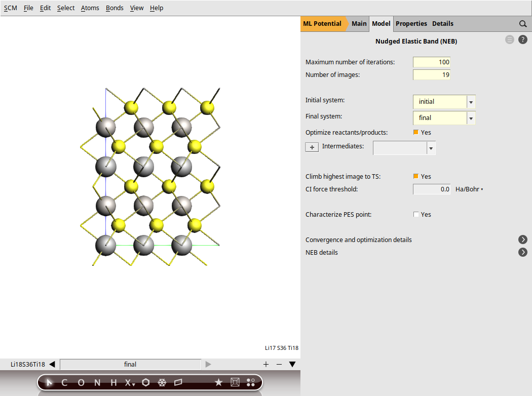
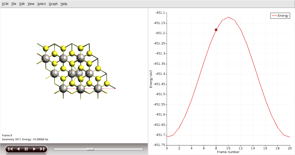
Run the calculation. This might take a few more minutes as AMS will perform a simultaneous optimization of all the 17 images by minimizing the forces parallel to the reaction path.
Once the calculation is finished, select LiTiS2_NEB in AMSjobs and click SCM → Movie. You can re-orient the crystal and use the slidebar under the molecule area to appreciate the diffusion along the minimum energy path. If you double click the y-axis label of the graph, you can switch to your preferred units. We found the activation energy EA = 0.59 eV.
NEB with Python
See the Li diffusion NEB scripting example.
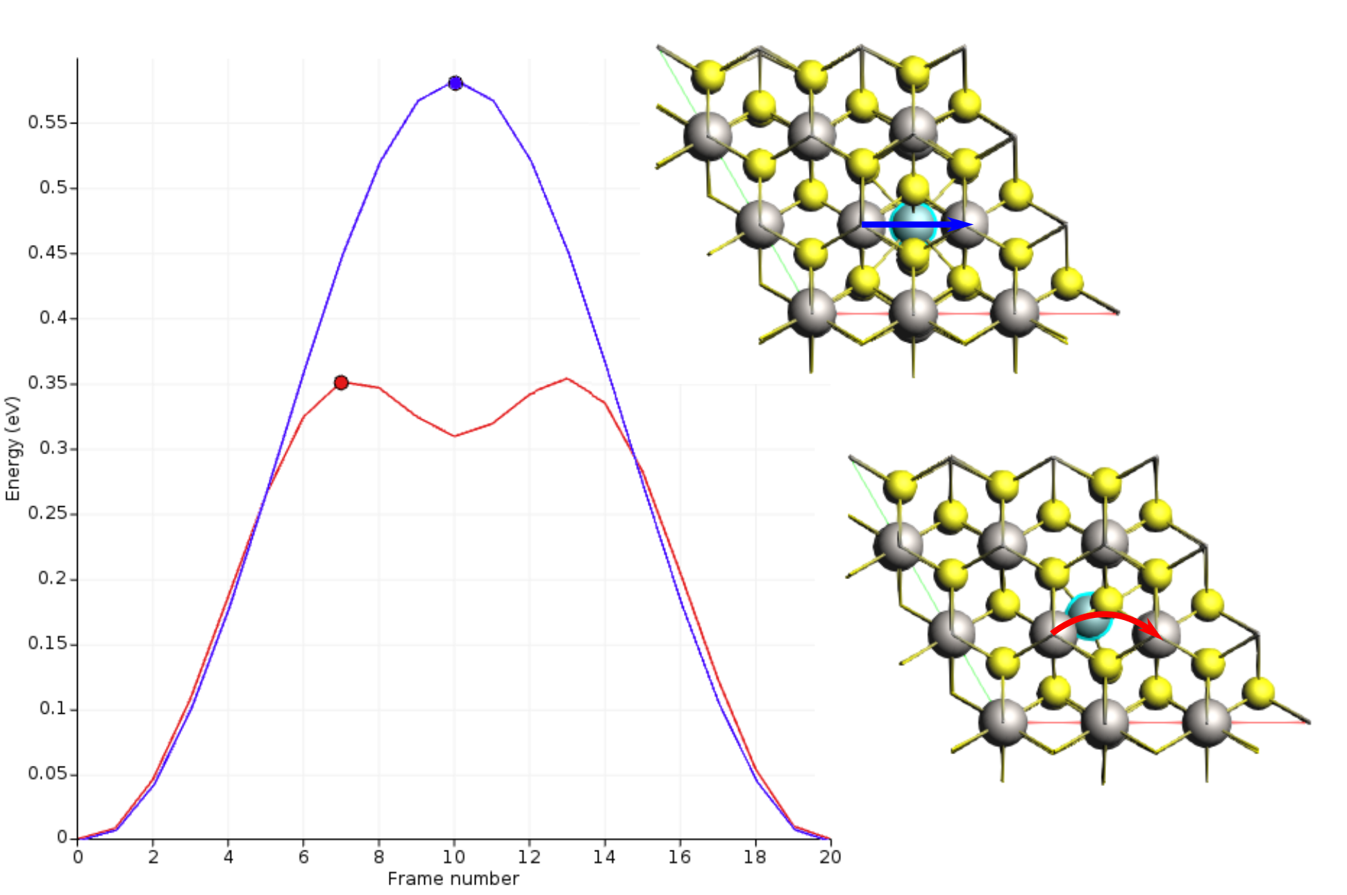
Li diffusion in LixTiS2
To explore the effect of lithium concentration on diffusion, begin with the structures from step 3. Remove the Li atom with index 9 for both the initial and final structures and at the end increase the NEB iterations to 500.
This change reduce the activation energy by approximately a factor of 2.
In the first case, the lithium migration trajectory was roughly linear.
The presence of the additional Li vacancy causes the path to curve, passing through a tetrahedral site and creating a shallow energy minimum.