Solvation beyond continuum solvation models: 3D-RISM

The three-dimensional reference interaction site model (3D-RISM) is a solvation model that can be viewed as a bridge between continuum solvation models such as COSMO and much more complex descriptions based on QM/MM molecular simulations. It describes the solvent in terms of interacting sites - such as H, O and CH3 in case of methanol - that are assigned point charges and Lennard Jones parameters, as is done in many force fields. Its output includes an estimate for the free energy of solvation as well as the averaged solvent (site) distribution around the solute. The AMS implementation 1 has recently been heavily supplemented 2 and features a self-consistent combination of the 3D-RISM approach and the (fitted) electron density obtained from DFT. In this combination, it can give insights into changes of the electronic structure of the solute upon solvation and related properties such as dipole moments and vertical excitation energies as required to investigate solvatochromism. 2

In this tutorial, we show how to run self-consistent 3D-RISM-SCF calculations and how to inspect the resulting solvent distributions using the example of acetone in water

Note

The 3D-RISM implementation is fully compatible with the calculation of analytical gradients, numerical frequencies (to verify the nature of a stationary point), vertical excitation energies and the calculation of EPR and NMR parameters (although specific MO contributions from the solvent are missing). See also the ADF manual on 3D-RISM.

Setting up and running the calculation

Load the structure of the acetone molecule from the molecules database and set up the calculation:

Start AMSinput

1. Press the button and search for Acetone and select C3H6O: Acetone (ADF)

2. Symmetrize the molecule by clicking the button

3. In the Main panel set Task to Single Point

4. Set XC functional to GGA:PBE

5. Set the Basis set to TZP

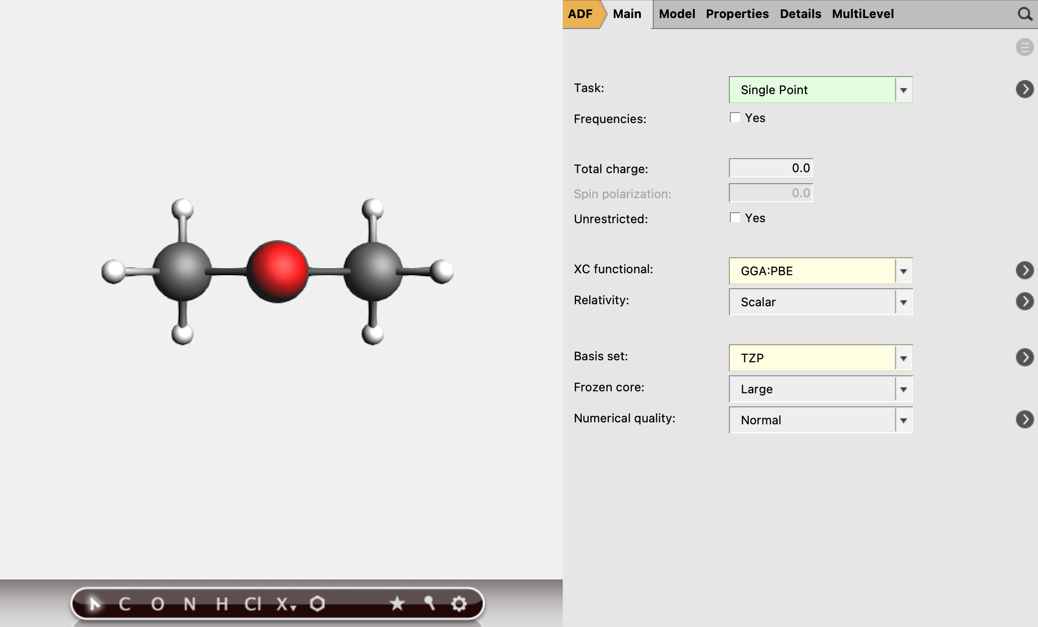
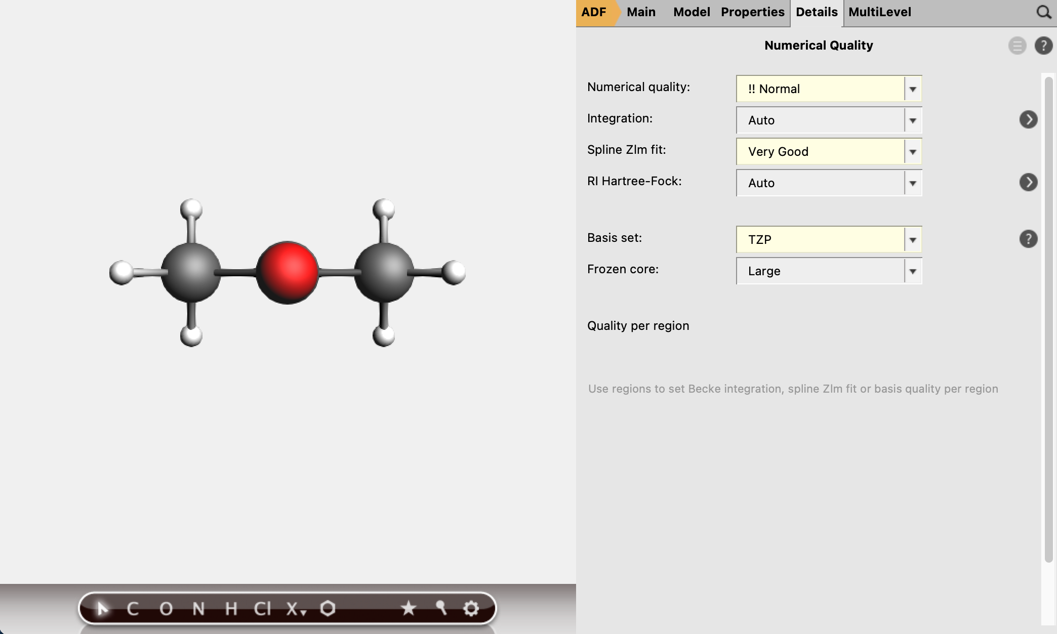
Since the 3D-RISM-SCF by default uses the fitted electron density to describe the electrostatic interaction between solvent and solute, it is highly recommended to increase the numerical quality of the density fit, especially for large molecules and when analytical gradients are computed. For this we set the Spline Zlm fit to better quality.

6. Move to Details → Numerical Quality and set Spline Zlm fit to Very Good

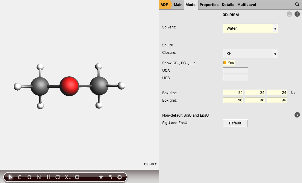
To set up the 3D-RISM part:

1. Move to Model → 3D-RISM and set Solvent to Water

2. In the same menu enable GF-, PC+, …

3. Set Box size to 24 24 24 Å

4. Set Box grid to 96 96 96

Note

The parameters used for the default solvents were taken from the SI of 2.

Note

The box - i.e., the cartesian grid, on which the 3D-RISM equations are solved - should extend far enough into space to allow for at least the first two or three solvation shells. Typically, adding 10 Å in each direction to the extent of the molecules is a good starting point. The grid spacing should not be above 0.5 Å (2 grid points per Å) and should best be below 0.33 Å (3 grid points per Å). The number of grid points has to be even and should have no prime factor larger than seven for optimal performance.

Now run the calculation:

1. File → Save, choose for example “Acetone_in_water” as name

2. File → Run

3. Wait for the calculation to finish, it should only take a few minutes

Results

A few interesting results have been written to the output file, such as free energy of solvation or the dipole moment of the molecule.

1. Open the output, SCM → Output

2. In AMSoutput search for “Corrections based on the calculated distribution functions”

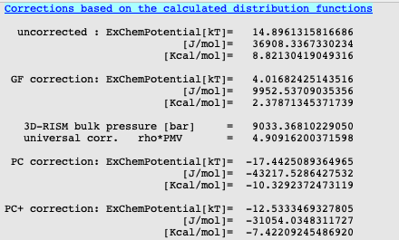
The calculated free energy of solvation of 8.82 kcal/mol is indeed much too positive for acetone in water (exp. -3.85 kcal/mol). The PC+ corrected value (-7.42 kcal/mol) gives the best agreement.

Note

For a formally correct free energy of solvation, the molecule should be optimized in both the gas phase and in solution and thermal corrections should be included!

For an inspection of dipole moment, search for “Dipole Moment” in AMSoutput.

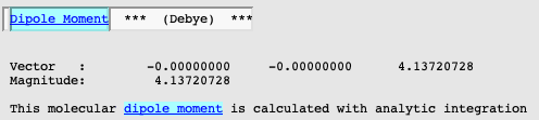
The dipole moment of 4.14 Debye is very close to the COSMO value (4.03 Debye) and shows the polarization of the C=O bond upon solvation (gas phase value at this level of theory: 2.87 Debye). Additional insight into this effect can be obtained from the solvent site distribution functions. They can be easily inspected using AMSview:

1. SCM → View

2. Add → Isosurface

3. Selected Field … → RISM…

4. Select the distribution of the second site (the water hydrogen) by clicking “RISM g(r) for site 2”

5. Enter a Isosurface value of 1.7

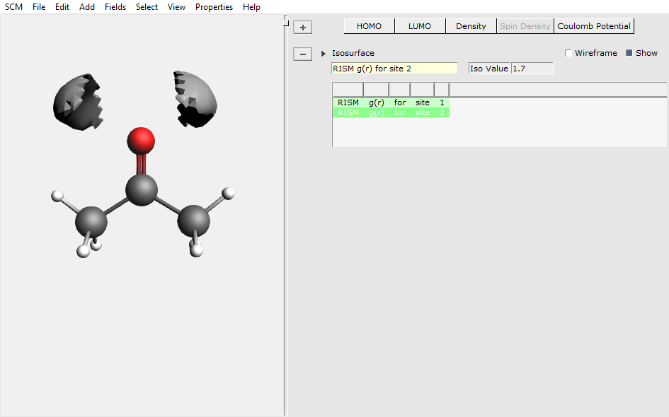
The isosurface shows the region in space, where the pair correlation function is above 1.7 – which corresponds to the local (site) density being 70 % larger than the average bulk density. The picture can straightforwardly be interpreted to show the hydrogen sited forming the hydrogen bonds to the oxygen lone pairs, which in turn explains the previously shown polarization of the C=O bond.

References

1

: Sergey Gusarov, Tom Ziegler and Andriy Kovalenko J. Phy. Chem. A 110, 6083-6090 (2006).

2(1,2,3)

: Marc Reimann and Martin Kaupp J. Phys. Chem. A 124, 7439-7452 (2020).