Defect formation energy

Point defects are omnipresent in materials and influence their electrical and optical properties. Understanding the formation of defects is critical for many industries in the area of physics and materials science. For example, this knowledge can be used to:

• design materials with specific and improved properties

• understand quality and ensure the reliability of materials

• gain insights into the manufacturing processes

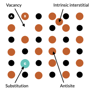
Therefore, first principles modeling of point defects has become an invaluable tool for understanding materials properties. Point defects range from simple vacancies to intrinsic or extrinsic substitutions and interstitials.

Because defects are usually present in very low amounts in crystalline materials (ppm), it is often of interest to examine the properties of a single defect in a pristine crystal. However, because of periodic boundary conditions, the size of the supercell must be sufficiently large to neglect the interactions between the periodic replicas of the defects. In the situation of charged defects, the strong and long-range nature of the Coulomb interaction between the localized charge distributions converges slowly. Consequently, the sizes of the supercells needed to produce accurate energies become excessively large. Thankfully, an ensemble of methods 2 3 have been proposed to correct for the spurious periodic interaction in small supercells to enable accurate computation of both neutral and charged defect formation energies, from first principles, and with reasonable computing resources.

In this tutorial we will learn how to compute defect formation energy in solids based on density functional theory. We will present the procedure to compute two types of defects:

• neutral defects

• charged defects

Note

In the following, we will use the indices p, 0, and q for perfect, neutral defect, and charged defect quantities. Moreover, to accelerate the calculations we will only consider unrelaxed defect cells, unless specified.

Note

To perform perform proper calculations on periodic systems, the number of kpoints should be wisely selected based on convergence tests, for each supercell size.

Neutral defects

Considering neutral defects, the defect formation energy can be expressed as:

\[E^f_0 = E_0 - E_p - \sum_i n_i\mu_i\]

with \(E^f_0\), \(E_0\), and \(E_p\) the defect formation energy, the total energy of the neutral defective structure, and the total energy of the perfect structure, respectively. The coefficients \(n_i\) represent the number of atoms of element \(i\) forming the defect (negative if removed, and positive if added) with chemical potentials \(\mu_i\), being reference energies for the added/removed atoms. Therefore, computing the neutral defect formation energy corresponds to finding the energies of the neutral defective structure, the perfect structure, and the chemical potentials of the atoms participating in the defect. Let’s have a look at some typical defects including vacancy, substitution, and interstitial. For example we will compute the defect formation energy corresponding to:

• C vacancy in diamond

• O substituted with N in MgO

• H interstitial in Si

Vacancy formation energy

We will demonstrate how to compute the vacancy formation energy in diamond with BAND.

Start AMSjobs

1. from the menu bar select SCM → New input

2. switch to the BAND engine →

3. from the menu bar select Edit → Crystal → Cubic → Diamond

4. in the pop-up window, select C from the Presets dropdown menu and click OK

5. from the menu bar select Edit → Crystal → Convert To Conventional Cell

6. from the menu bar select Edit → Crystal → Generate super cell..

7. click OK in the Dialog Window to generate a 3x3x3 supercell

8. click next to Numerical quality → K-space and select Good from the dropdown menu

Note

There is a shortcut to Edit → Crystal (in the menu bar) by clicking the icon at the bottom of the molecule panel in AMSinput.

Note

It can also be a good idea to enforce symmetry of the crystal in order to optimize the performances of the DFT calculation.

Furthermore, we will mark the position of the future vacancy by creating a region containing the C atoms that we will delete in the next calculation. This will ensure the exact same number of symmetry operators in all the calculations.

1. select a C atom

2. go to Model → Regions

3. click the + symbol left of Regions

4. rename the region as vacancy

Later on we want to align the potential of a charged defect, and that is why two extra steps are needed

1. Set the origin to the C atom in the vacancy region Edit → Set Origin, because we want to align the potential far away from the vacancy, at the edge of the unit cell.

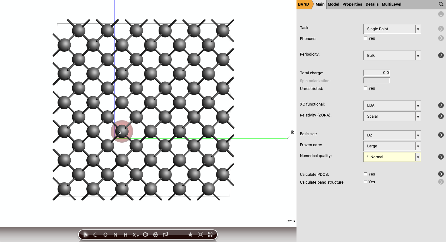
2. Using the looking glass icon (), search for the option UpdateStdVec, and disable it (Programmer%UpdateStdVec) in the Details → Expert BAND panel. Otherwise the systems may be shifted with respect to each other, spoiling the alignment, see for instance Fig. 1.

You can keep all defaults parameters, save the job as C_diamond_3x3x3_p and run the calculation. This corresponds to running a single point DFT calculation with the LDA exchange-correlation potential and the DZ basis set. The number of k-points was set to Good, which will result in 3 kpoints along each lattice direction.

Once the calculation is over, we can compute the energy of the defective cell.

1. from AMSjobs click the BAND icon next to the job you just executed to open AMSinput

2. select the C atom that we previously tagged by the Regions by left-clicking on it and delete the atom with the delete key

3. you can also delete the region from Model → Regions and then click the - symbol left the vacancy region

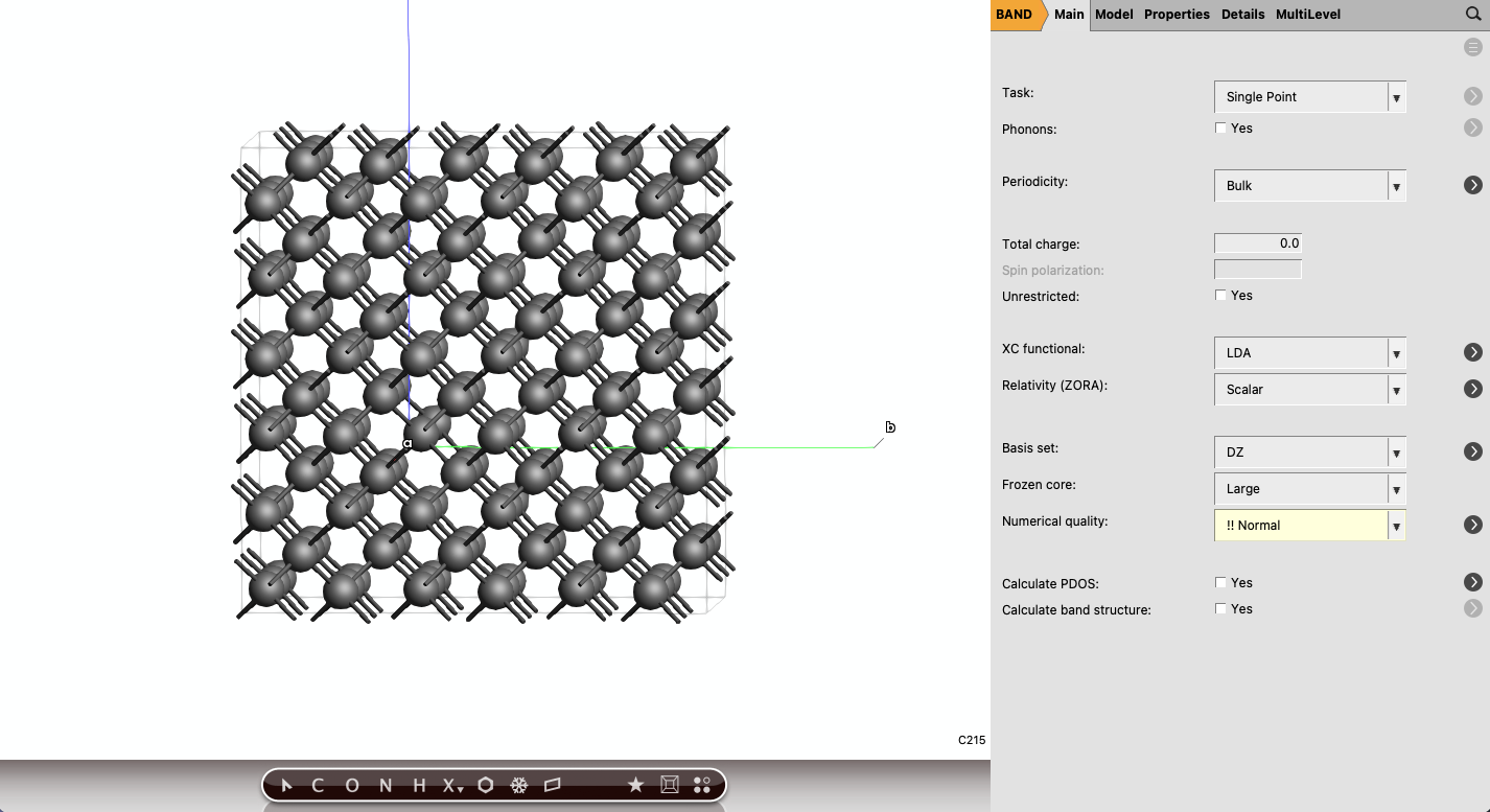
Save the job as C_diamond_3x3x3_0 and run the calculation.

To create the vacancy, we have simply removed a carbon atom, therefore, \(-\sum_i n_i\mu_i = +\mu_C\). In general, the chemical potential of the atoms that participate in the defects are taken as the energy of that atom in its ground state structure. In the case of carbon, we can use the total energy of the diamond structure as reference.

We can summarize the results in the table below:

Table 3 Summary of the total energies computed with LDA for C.

Calculations	Perfect diamond (p)	Diamond vacancy (0)
Number of atoms	216	215
Energy (eV)	-2118.32	-2099.94

The neutral vacancy formation energy in C diamond can be calculated as:

\[E^f_0 = E_0 - E_p +\mu_C = -2099.94 - -2118.32 + -2118.32/216 = 8.57 \text{ eV}\]

It is interesting to appreciate how increasing the supercell affects the vacancy formation energy. You can repeat the previous calculations in a smaller (2x2x2) and larger (4x4x4 and 5x5x5) supercells.

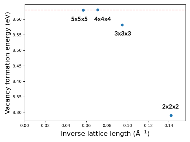
We can conclude that from the supercell size of 4x4x4, the vacancy interaction becomes negligible.

Some considerations

Here follow some thoughts on the choice of the chemical potentials and the k-grid.

Chemical potential

The chemical potential represents the energy of a single atom being taken from or added to some reservoir. As such there is some arbitrariness, and it is important to specify how the reference systems are chosen. Above we have chosen for the Carbon atom the energy of the Diamond crystal per atom. Alternative choices could have been the energy per atom in Graphite, or a Bucky ball. Sometimes combinations are taken: for instance in the work of Komsa 2 the chemical potential of Ga is defined as the energy of the GaAs crystal minus the one from As

\[\mu_\text{Ga} = \mu_\text{GaAs} - \mu_\text{As}\]

In an experimental setup the chemical potential may depend on the temperature and pressure.

K-points

As neutral defects formation energies converge quite quickly with super cell size no super cell extrapolation is needed, and it may be beneficial to use the GammaOnly k-grid (with only one k-point). For small super cells the GammaOnly calculations are far from k-space converged, but you can go to bigger super cells, that may be cheaper to calculate than a smaller unit cell with more k-points. With increasing super cell size, the GammaOnly grid becomes progressively more accurate.

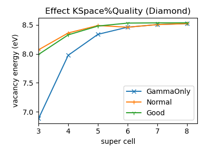
In the figure we see the vacancy formation energy for several choices of the KSpace%Quality (obtained with DFTB). While for the 4x4x4 super cell (abbreviated as super cell 4) the energy may be k-space converged with KSpace%Quality=Good, a better value is obtained with GammaOnly at super cell=6. The latter may be faster.

Substitution

In this second example, we will explore the case of a nitrogen substitution in the oxide MgO. We start with the perfect supercell.

1. in the menu bar of AMSjobs select SCM → New input

2. switch to the QE engine →

3. click the magnifier icon and search for MgO

4. Edit → Crystal → Convert To Conventional Cell

5. Edit → Crystal → Generate super cell..

6. click OK in the Dialog Window to generate a 2x2x2 supercell

7. set the Wavefunction energy cutoff to 60.0 Ry

8. set 2 K-points in each dimension

9. select PZ (LDA) next to XC and uspp next to Type

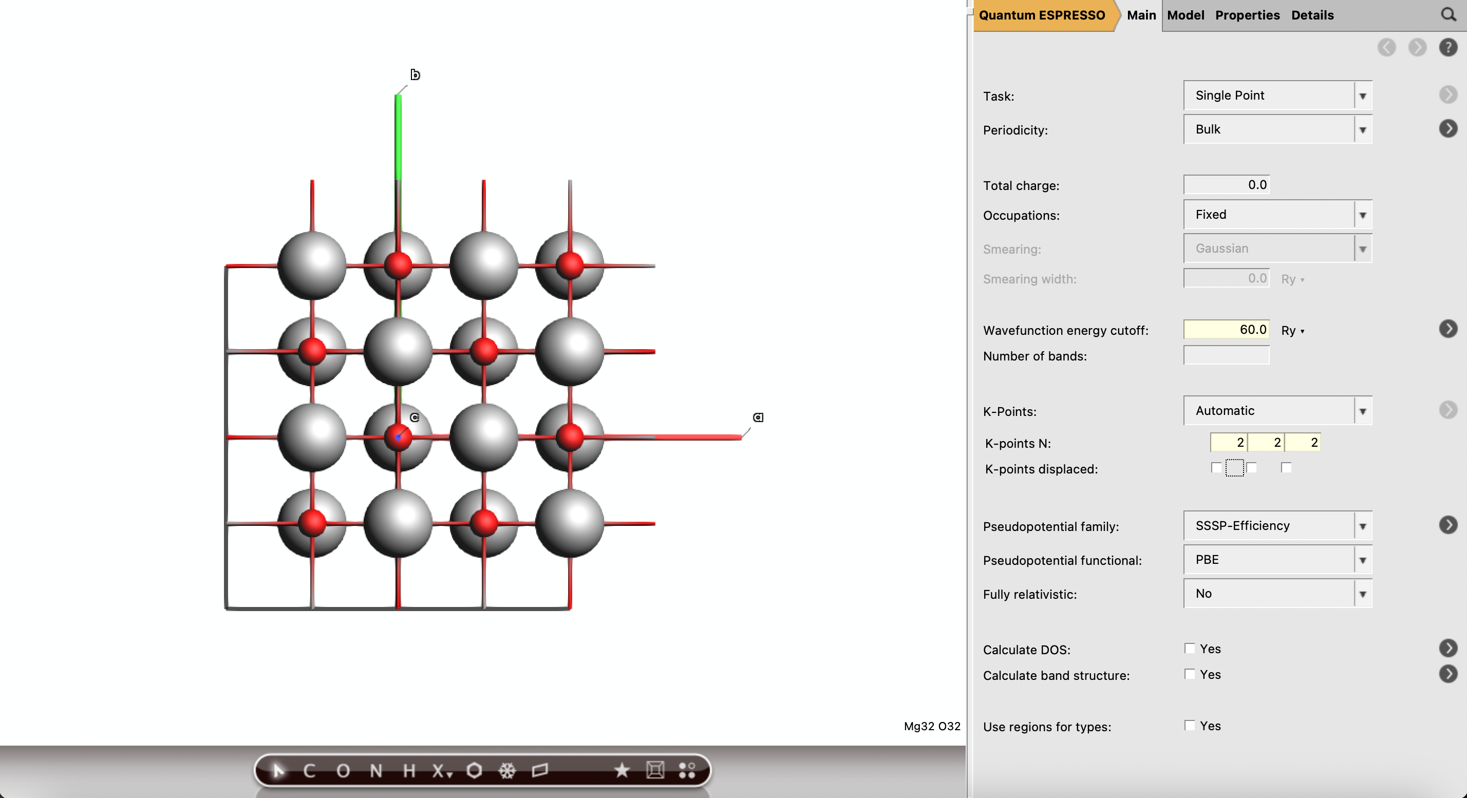
Save the job as MgO_2x2x2_p and run the calculation. With these settings, we are going to perform a single point calculation with QE with a 60 Ry kinetic energy cutoff, 2x2x2 k-grid, at the LDA level with ultra-soft pseudo potentials. Once the calculation is finished, you can reopen the calculation to prepare the defective cell.

1. in AMSjobs click the QE icon next to MgO_2x2x2_p to open the previous calculation

2. select an O atom and click Atoms → Change Atom Type and select N (ignore the warnings)

3. Select Collinear next to Magnetization

4. Go to Model → Magnetization and fix the total magnetization to 1

Note

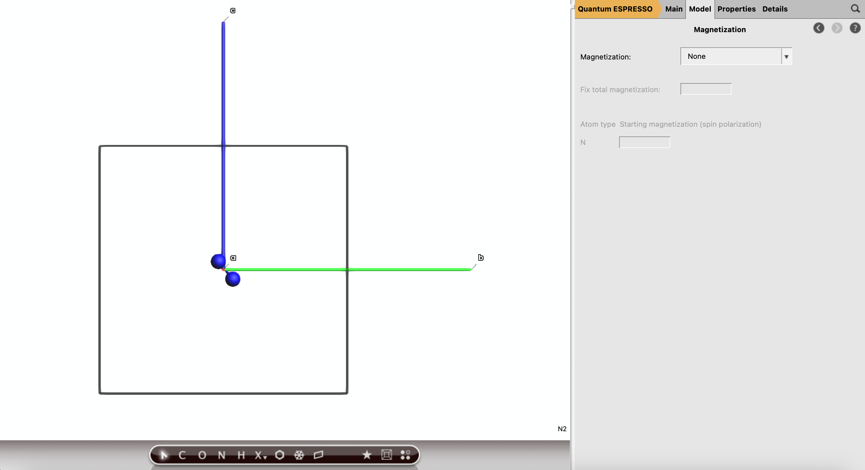
Here we need to set the magnetization because we now have an odd number of electrons. It is also possible to perform a charged state calculation with an even number of electron (see below).

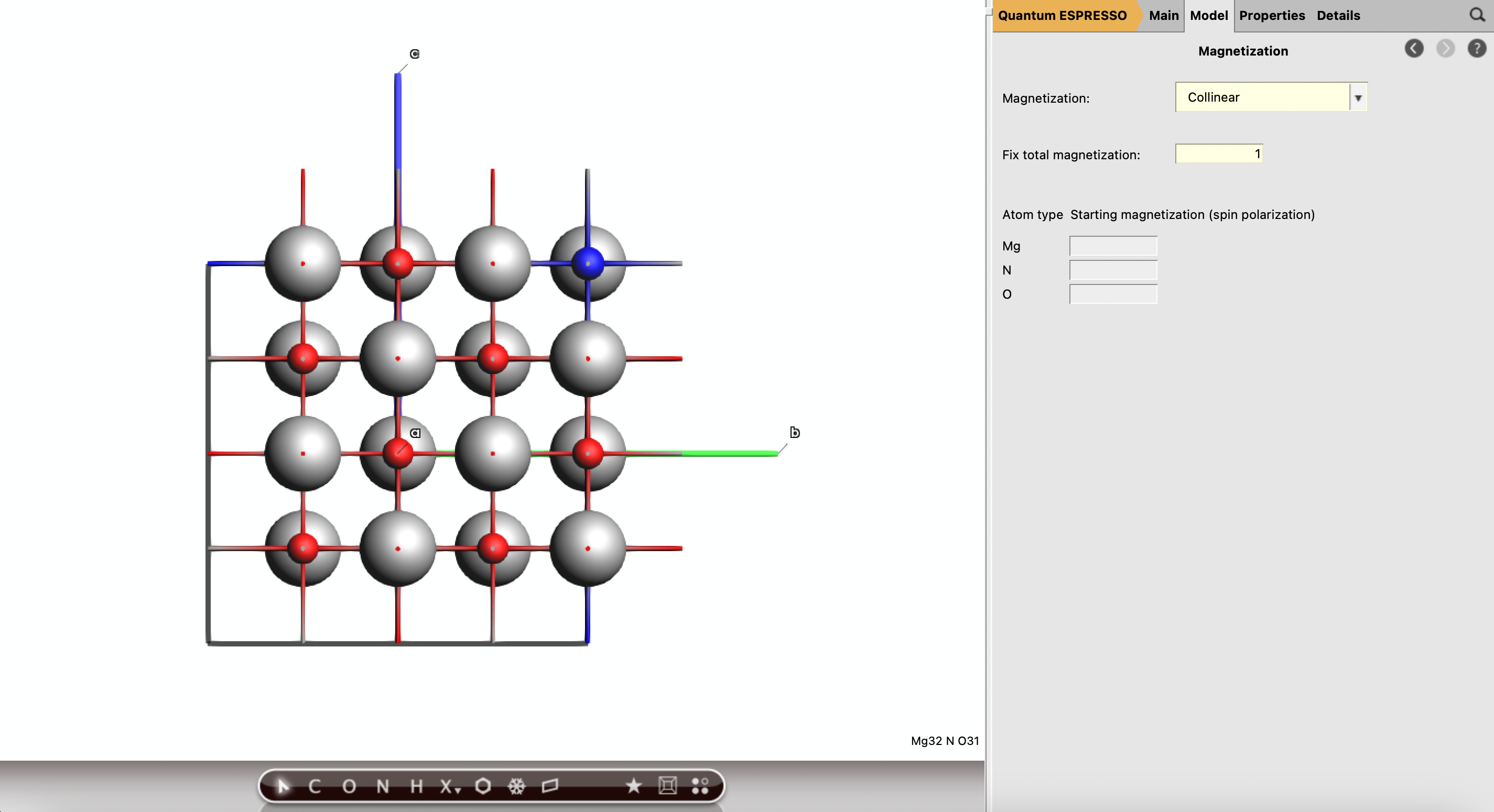
Save the job as MgO_2x2x2_OsubN_0 and run the calculation.

Now we need 2 more calculations to compute the chemical potential of O and N. The ground state of oxygen is taken as the energy per atom of the \(\text{O}_2\) molecule and that of nitrogen is taken as the energy per atom of the \(\text{N}_2\) molecule. We can start from the MgO_2x2x2_OsubN_0 calculation in order to keep settings from the previous job.

1. in AMSjobs click the QE icon next to MgO_2x2x2_OsubN_0

2. select all the atoms and delete them (hold shift and drag the mouse over the crystal and tap delete)

3. go to Model → Lattice, set the diagonal of the Lattice vectors to 12 Å

4. select the O icon and click twice in the molecule area followed by the esc key

5. select the two O atoms and set the distance to 121 pm (you can either input the distance in the input cell at the bottom-right of the molecule area or adjust the distance with the slide bar at the bottom of the molecule area)

6. set the Task to Geometry Optimization

7. from the Magnetization tab fix the total magnetization to 2

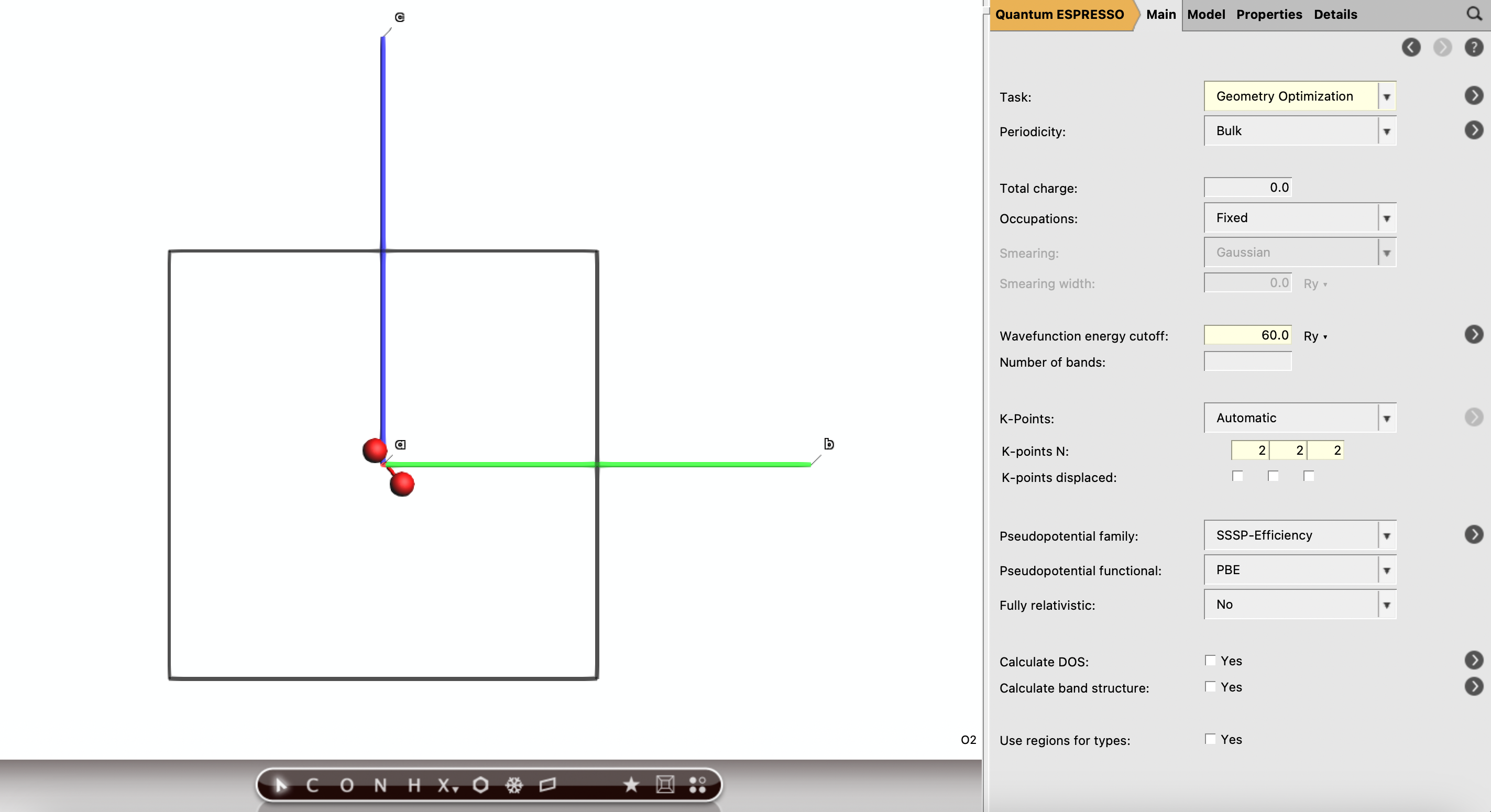
Save the file as O2 (File -> Save As..) and run the calculation. Once finished, open the calculation in AMSinput to create the \(\text{N}_2\) run.

1. in AMSjobs click the QE icon next to O2

2. select all atoms and click Atoms → Change Atom Type to N

3. select the two N atoms and set the distance to 110 pm

4. set the Magnetization to None

Save the job to N2 and run the calculation. We can summarize the results in the table below:

Table 4 Summary of the total energies computed with LDA for MgO.

Calculations	MgO (p)	MgO with N substituted (0)	\(O_2\) molecule	\(N_2\) molecule
Number of atoms	64	63	2	2
Energy (Ry)	-5043.979	-5031.537	-64.221	-40.253

To create the substitution, we have removed a O atom and added a N atom, therefore, \(-\sum_i n_i\mu_i = +\mu_O - \mu_N\). The substitution formation energy in MgO can be calculated as:

\[E^f_0 = E_0 - E_p +\mu_O - \mu_N = -5031.537 - -5043.979 +-64.221/2 - -40.253/2 = 0.458 \text{ Ry}\]

We found that the formation energy corresponding to an oxygen substituted with nitrogen in MgO is 6.23 eV.

Note

The supercell size for this example is probably too small to neglet the defect interaction between periodic images, and one should check convergence of the defect formation energy as a function of supercell size.

You can also verify that the numbers of kpoints used for the calculations of the defect formation energy were sufficient by repeating the calculation with various number of kpoints. This can be achieved with this PLAMS script

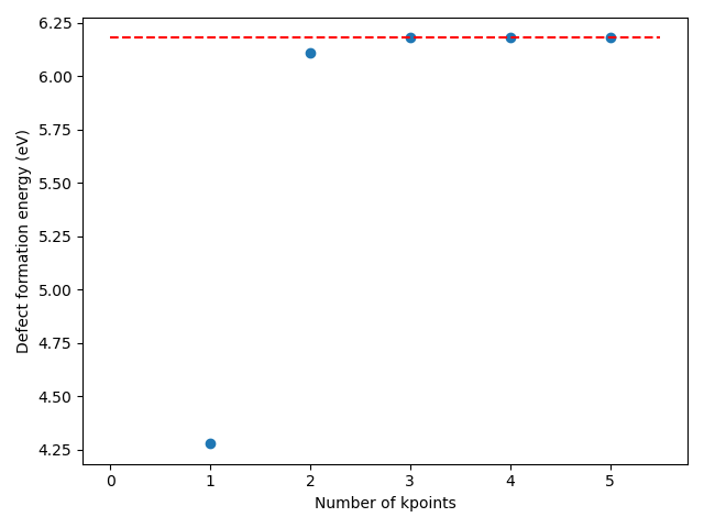
Based on the above convergence test, we can conclude that using a 2x2x2 k-grid to described the defect formation energy of N substituted MgO leads an approximate error of ~0.05 eV as compared to a fine 5x5x5 k-grid. Therefore, a 3x3x3 k-grid is recommended.

Band and DFTB calculations

Remember that we are interested in the super cell limit. If you use the GammaOnly k-grid the super cell dependence of the substitution energy is

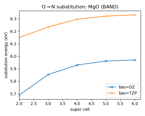
We can conclude that BAND predicts a super cell converged substitution energy of about 6 eV with a DZ basis. Using a TZP basis set this becomes about 6.35 eV.

The band procedure can be summarized as.

• Start from the minimal cell of MgO

• Make a larger super cell

• Make a region for the atom that you want to substitute

• Use the GammaOnly k-grid.

• Use the Unrestricted keyword

• Run the pristine and substituted system

• The N2 and O2 molecules can be calculated without an artificial lattice, i.e. as true molecules.

• There is no need to set the spin explicitly. The Unrestricted is only really needed for the substituted systems and for the O2 molecule.

If you try this with DFTB a very different value is obtained of -30 eV. DFTB is not able to describe substitution energies.

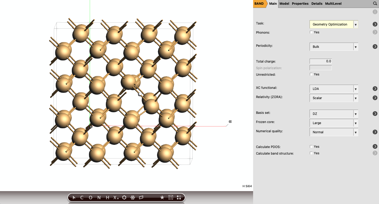
Extrinsic interstitial

For the last example, we will compute the formation energy of a neutral H interstitial in Silicon. Neutral H interstitial will seek out the regions of highest electronic charge density, which corresponds in Silicon crystals at the midway between two Si atoms. Let’s start by computing the energy of the perfect supercell.

Start AMSjobs

1. from the menu bar select SCM → New input

2. switch to the BAND engine →

3. from the menu bar select Edit → Crystal → Cubic → Diamond

4. in the pop-up window, select Si from the Presets dropdown menu and click OK

5. from the menu bar select Edit → Crystal → Convert To Conventional Cell

6. from the menu bar select Edit → Crystal → Generate super cell..

7. click OK in the Dialog Window to generate a 2x2x2 supercell

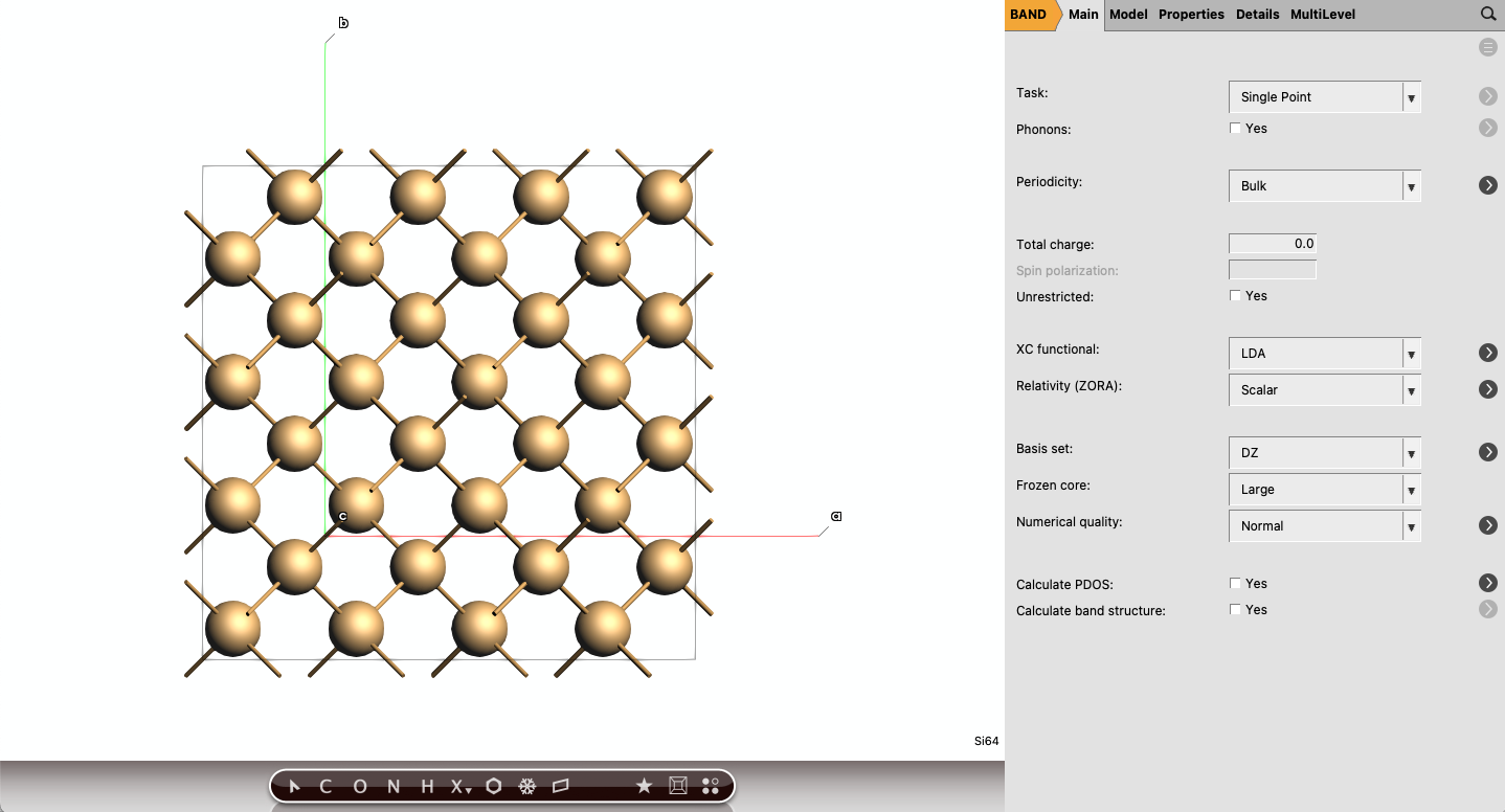
Save the job to Silicon_2x2x2_p and run the calculation. We can prepare the defective cell from the previous settings.

1. from AMSjobs click the BAND icon next to the job you just executed to open AMSinput

2. select two bonded Si atoms by left-clicking on them with the shift key pressed in

3. from the Atoms menu select Add Dummy At Center Of Selection

4. left-click the dummy atom and select Atoms → Change Atom Type, and choose H

5. select the Task Geometry Optimization

Before running the geometry optimization, we need to make some room for the H interstitial. This can be achieved as follow.

1. select one of the bonded Si and move it slightly away from the H interstitial by right-clicking on it and moving the mouse in the desired direction

2. select the second bonded Si and move it slightly away from the H interstitial

Ideally, you would like the distance between the H and neighbors Si to be 1.6 Å.

Save the job to Silicon_2x2x2_0 and run the calculation. Now we can calculate the chemical potential of hydrogen, taken as the total energy per atom for \(\text{H}_2\).

1. from AMSjobs click the BAND icon next to the job you just executed to open AMSinput

2. delete all the atoms in the supercell

3. create two hydrogen atoms and set their distance to 0.77 Å

4. set the Periodicity to None

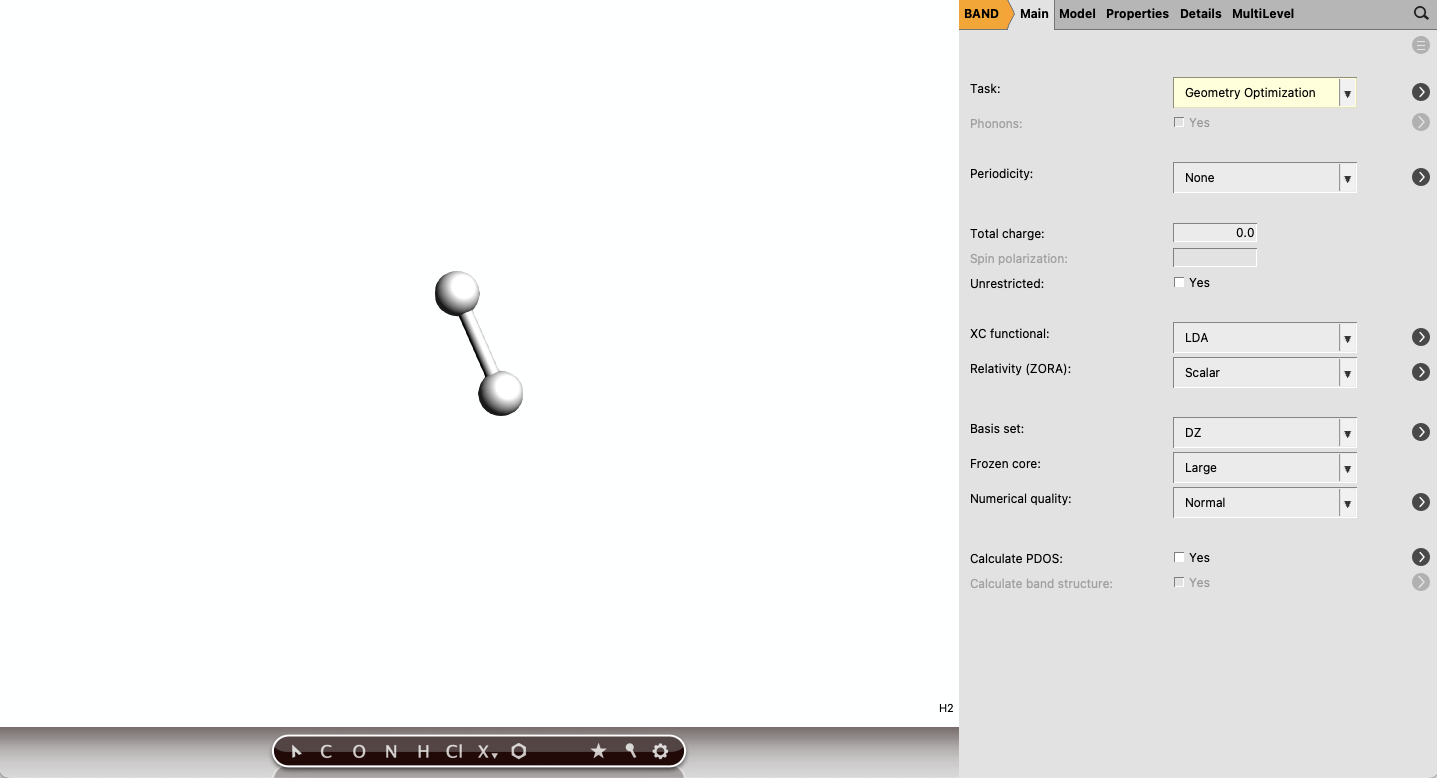
Save the job to H2 and run the calculation. We can summarize the results in the table below:

Table 5 Summary of the total energies computed with LDA for Silicon.

Calculations	Silicon (p)	Silicon with H interstitial (0)	\(H_2\) molecule
Number of atoms	64	65	2
Energy (eV)	-338.7376	-340.3065	-6.6213

To create the interstitial, we have added a H atom, therefore, \(-\sum_i n_i\mu_i = - \mu_H\). The interstitial formation energy in Silicon can be calculated as:

\[E^f_0 = E_0 - E_p - \mu_H = -340.3065 - -338.7376 - -6.6213/2 = 1.74 \text{ eV}\]

Charged defects

Considering now charged defects, the defect formation energy can be expressed as:2

\[E^f_q = E_q - E_p + E_\text{corr} - \sum_i n_i\mu_i + q[\epsilon_F + \Delta V_{0/p}]\]

with \(E^f_q\) and \(E_q\), the charged defect formation energy and the total energy of the charged defective structure, respectively. \(E_\text{corr}\) is the finite-size supercell correction that we will ignore first and discuss later. \(q\) is the charge of the defect, \(\epsilon_F\) the fermi energy, and \(\Delta V_{0/p}\) is a term used to align the electrostatic potential of the perfect and neutral defective supercells. Indeed, the electrostatic potential between the perfect and neutral defective supercells can be slightly different and is estimated by the difference of the electrostatic potential away from the defect 2. The term \(q\epsilon_F\) here is equivalent to the chemical potential of the electron which is added if the charge is positive or subtracted if the charge is negative, similar to the \(\sum_i n_i\mu_i\) term for the atoms.

Note

Note that because of the periodic boundary conditions it is not possible to compute the energy of a charged supercell and most engines will introduce a compensating homogenous background charge to neutralize the total charge.

Note

Because of the computational limitations of density functional theory, it is not possible to perform a supercell calculation with similar concentration as in the real crystal. This limitation leads to a highly concentrated defect in the supercell. As we have seen above, in the case of neutral defects, the choice of a reasonably large supercell is enough to limit the periodic interactions between defects. However, because of the long-range effect of Coulomb interaction, the proper calculation of a charged defect must be extrapolated to an infinitely large supercell.

We provide below two examples based on diamond to compute the formation energy of charged C vacancy using:

• the supercell method

• finite-size supercell correction

Comparing potentials of different geometries

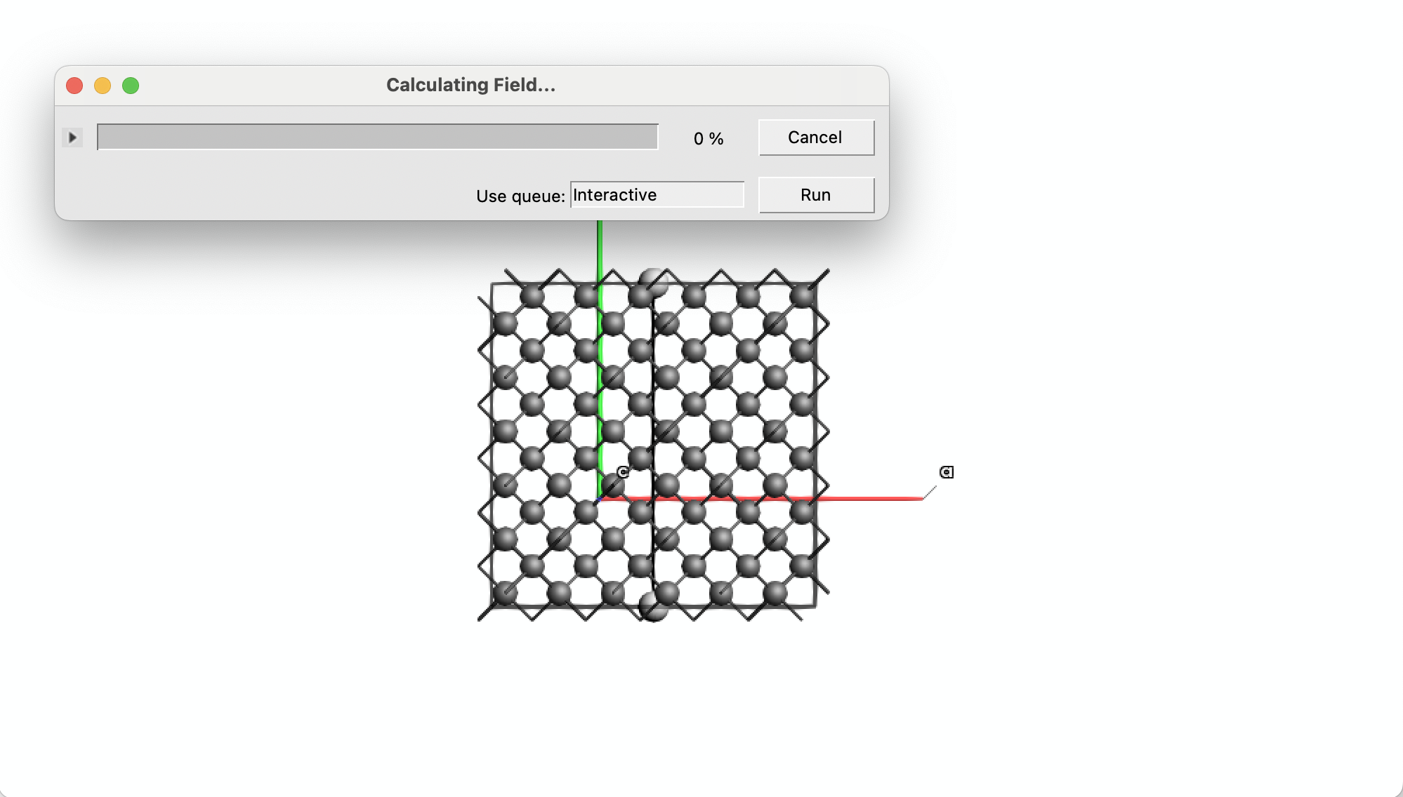
For the calculation of \(\Delta V_{0/p}\) we determine the difference in the coulomb potential of the defect and the pristine system. By default band may shift a system, to maximize the symmetry. If this shift is different for the two systems we get a wrong result. To avoid this we have to use Programmer%UpdateStdVec=No.

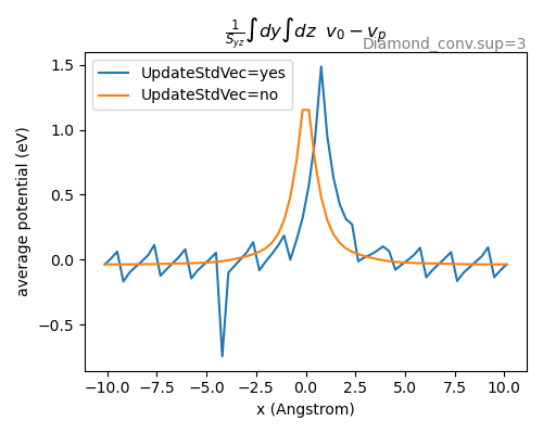
Fig. 1 The plane averaged potential difference requires that both systems have the same origin, otherwise a wrong result may be obtained, as shown with the blue curve. To avoid letting band change the origin use Programmer%UpdateStdVec=No.

Supercell method

The supercell method consists of computing the formation energy of charged defects for various supercell sizes, and to extrapolate the defect formation energy of an isolated defect in the limit of infinite supercell size. One of the major drawback of this method is that it requires the calculations of at least 3 supercell sizes.

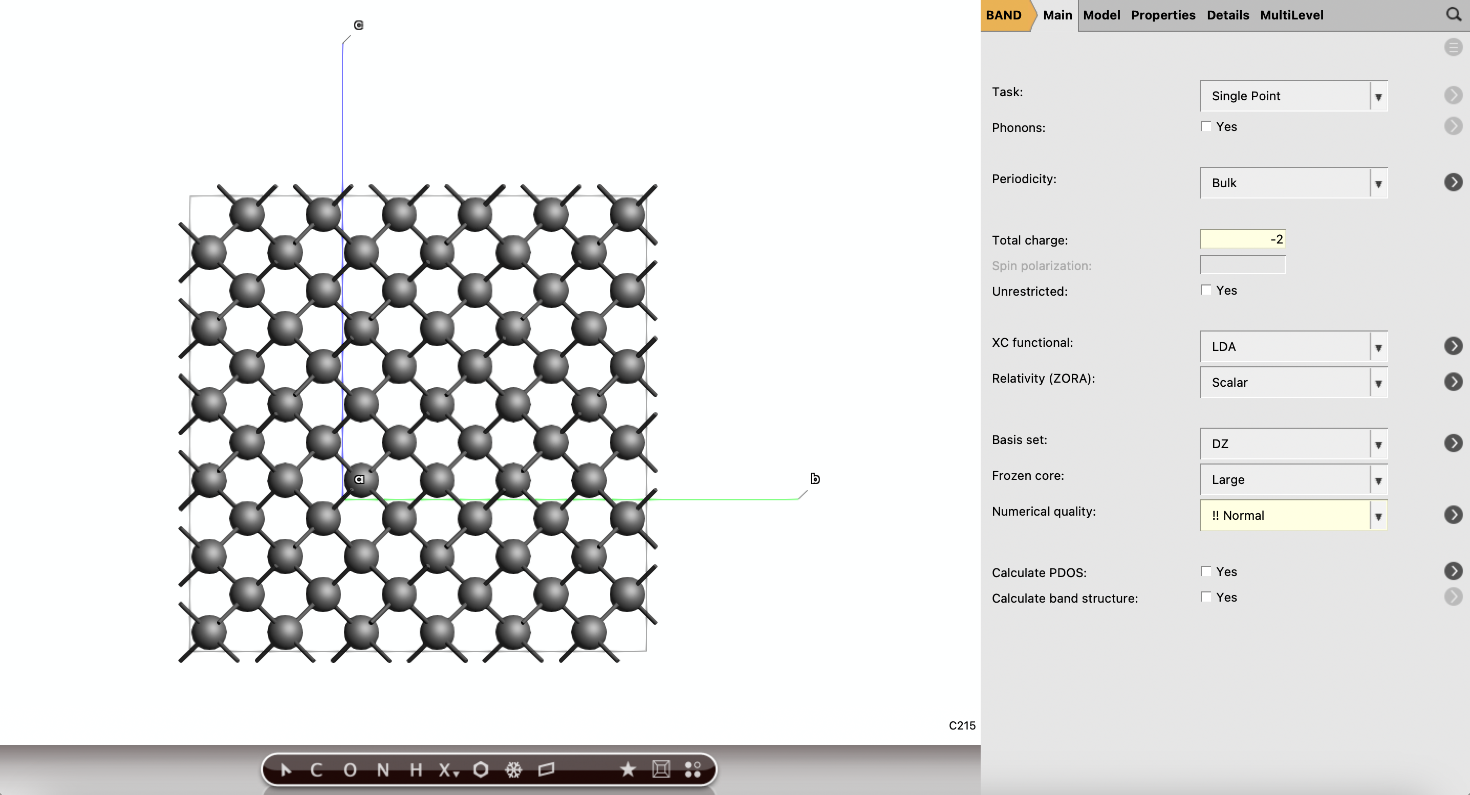
To illustrate the procedure, we will compute the -2 charged vacancy formation energy in diamond (\(V^{-2}\)). We need to perform the calculations corresponding to neutral perfect, neutral defect, and charged defect supercells. We already performed calculations for neutral perfect and neutral defect cells. We can just reopen the neutral defect and set the charge to -2.

1. from AMSjobs click the BAND icon next to the job we saved as C_diamond_3x3x3_0

2. set the Total charge to -2

Save the job to C_diamond_3x3x3_q and run it. You can approve when the pop-up will tell you that a neutralizing density will be added to the charged density.

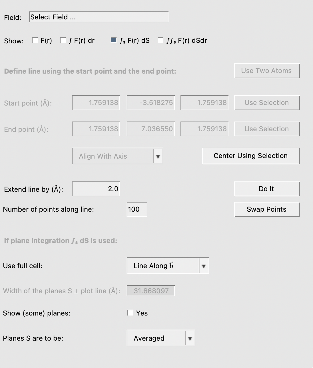
Looking at the charged defect formation energy equation, the energies can be extracted as usual, and the Fermi energy will be approximated to the energy of the top of the valence band (~ -7 eV). We just need to extract the potential alignment term \(V_{0/p}\) between the neutral perfect and neutral defective cells. We will compute and save the planar averaged of the Coulomb potential and execute a Python script to extract the value of \(V_{0/p}\).

1. in AMSjobs select the neutral perfect job and click SCM → View

2. select Add → Graph Along Line

3. next the Use full cell select Line along b in the dropdown menu. (Line along a and along c are equally good choices, as the cell is a cube)

4. select Averaged next to Planes S are to be

Now switch back to the AMSview window to define which quantity we want to averaged.

1. in AMSview check the button next to \(\int_S F(r) dS\) and uncheck F(r)

2. click Select Fields → Potential → Coulomb Potential

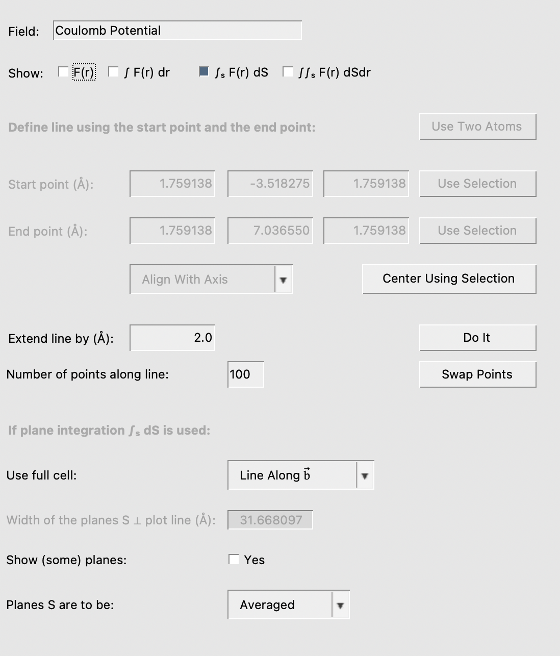
Wait for the planar averaged to be completed. In the Coulomb Potential Line Plot window, click the Save XY Values and save the plot as C_diamond_3x3x3_p_coul.xy.

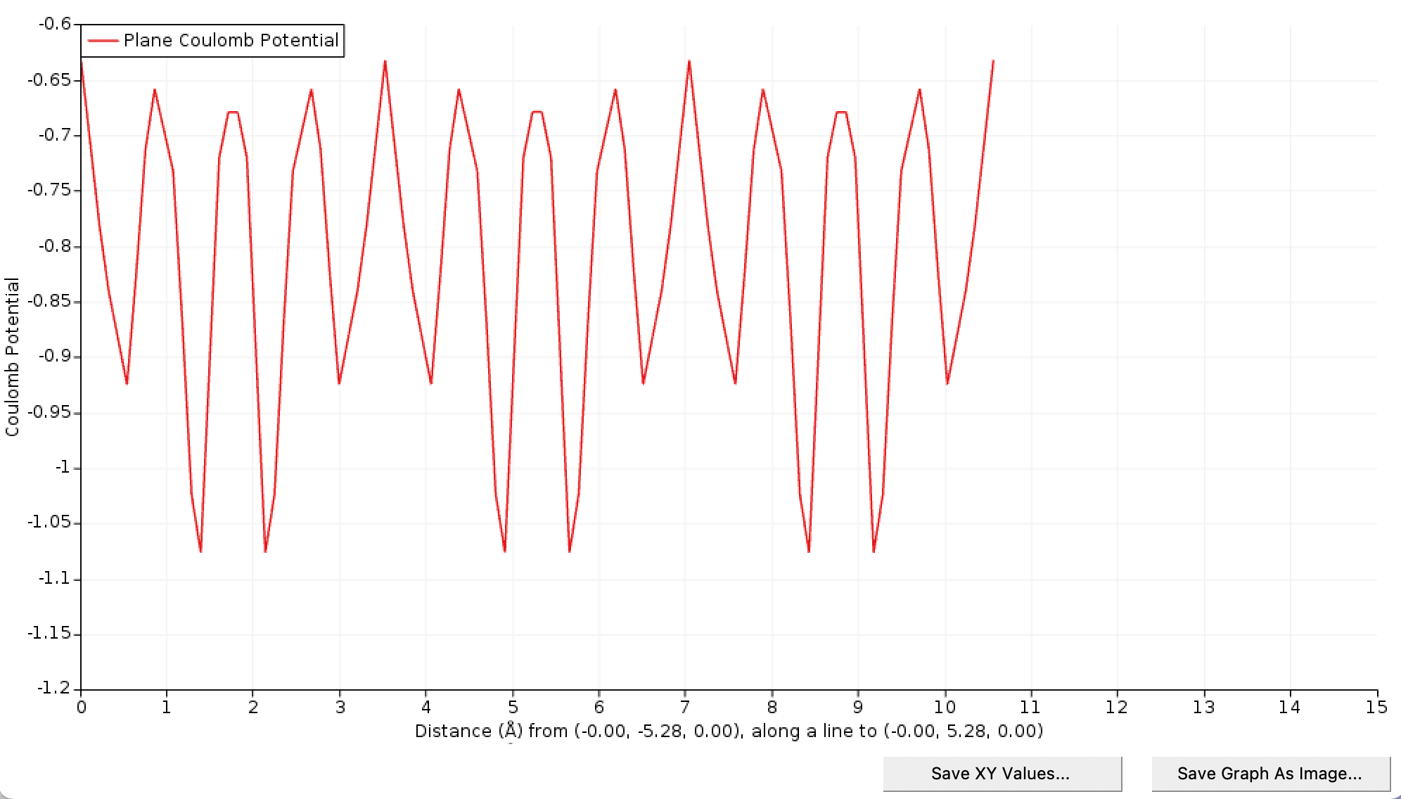
Reproduce the previous steps to extract the Coulomb potential of the neutral defective cell and save the graph as C_diamond_3x3x3_0_coul.xy. Plotting both potentials (using for instance a spreadsheet program) we see that the pristine and defect potentials are very similar with some difference near the center of the cell, exactly as hoped for

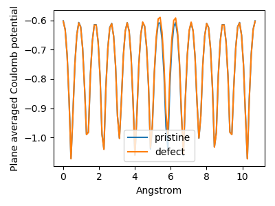
Download this Python script and execute it in the same directory of the two XY files saved previously.

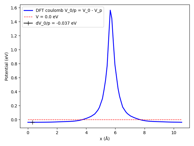
This is the Coulomb potential corresponding to the neutral vacancy. The value of the potential difference away from the vacancy gives us \(V_{0/p}\) which is also outputted by the Python script. We can now summarize the calculations.

\[E^f_q = E_q - E_p - \sum_i n_i\mu_i + q[\epsilon_F + \Delta V_{0/p}]\]

Table 6 Summary of the total energies computed with LDA for C (all in eV).

Calculations	C (p)	C (0)	C (q)	E VB (p)	\(ΔV_{q/0}\)	\(E^f_q\)
2x2x2	-627.68	-609.58	-620.57	-7	-0.097	11.49
3x3x3	-2118.32	-2099.94	-2110.44	-7	-0.037	12.15
4x4x4	-5021.28	-5002.84	-5013.03	-7	-0.005	12.45
5x5x5	-9807.05	-9788.61	-9798.59	-7	-0.011	12.68

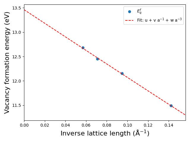
The supercell method consists in reproducing the previous calculations within various supercell sizes. We performed calculations in 2x2x2 and 4x4x4 supercells and we provide below the plot of the charged defect formation energy as a function of lattice parameter. By extrapolation, we find the isolated defect formation energy to be of 13.5 eV.

Note

Comparing the previous charged defect formation energy and the neutral defect formation energy scalings we can appreciate the strong long-range effect of the charge Coulomb potential compared to that of the neutral defect. Indeed, while a 4x4x4 supercell was large enough to compute an accurate neutral defect formation energy in diamond, here we see that the same supercell is still off by almost 1 eV for charged defect!

Finite-size supercell correction

Several flavors of finite-size supercell corrections have been proposed and we will describe the scheme of Freysoldt, Neugebauer, and Van de Walle (FNV) 1. The idea of the finite-size supercell correction is that since direct first principle calculations of the charged defect formation energy with various supercell sizes is computer intensive, one would only perform calculations in a relatively large supercell and an approximated model will be used to correct for the finite-size supercell interaction including the proper isolated defect interactions. In the FNV scheme, the defect density is approximated with a Gaussian function and the corresponding potential and energy are calculated by solving the Poisson equation. The correction term is defined as

\[E_\text{corr} = E_{lat} - q\Delta V_{q/0}\]

where \(E_{lat}\) corresponds to the lattice finite-size correction and \(\Delta V_{q/0}\) the potential alignment between the model and the DFT calculation. The model supercell calculation for \(E_{lat}\) involves solving the Poisson equation for the periodic model potential, \(V_{lat}(r)\).

\[\nabla\cdot [\epsilon (r)\nabla V_{lat}(r)] = -4\pi\rho(r)\]

with \(\epsilon (r)\) the dielectric tensor profile of the materials and \(\rho(r)\) the model charge distribution. The dielectric tensor can be computed from density functional theory, as described in this tutorial. In a 3D bulk system with an isotropic dielectric, \(V_{lat}(r)\) can be obtained as:

\[V_{lat}(G) = \frac{4\pi \rho(G)}{\epsilon |G|^2}\]

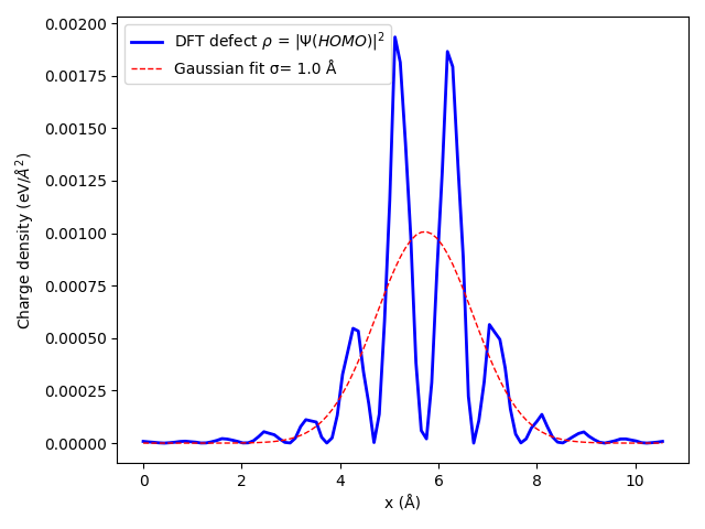
The number of G vectors used in the calculation is determined by an energy cutoff. To best define the charge density of the model Gaussian distribution, one needs the width of the distribution. This can be obtained by fitting the DFT defect charge density. First, you need to identify the molecular orbital of the defect. This can be achieved by looking at the DOS (or even better at the band structure).

1. in AMSjobs select the charged defect job and click SCM → DOS

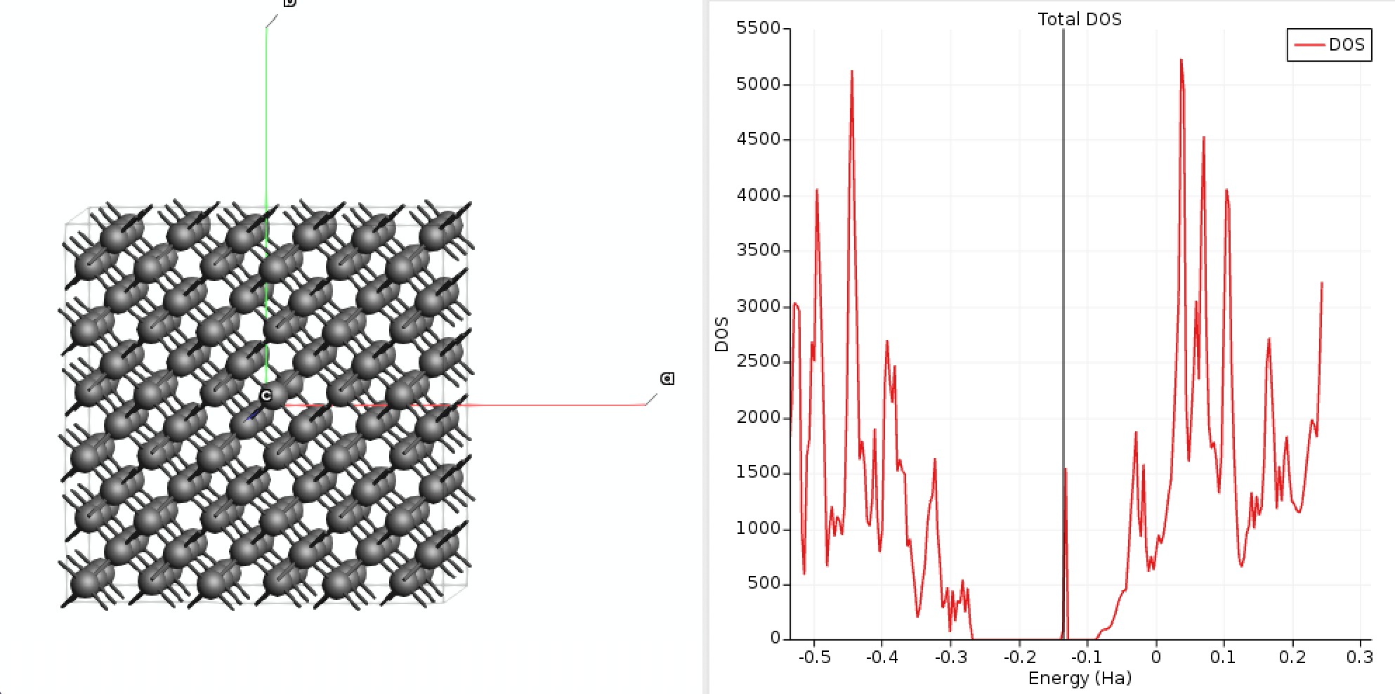
We can clearly see a state in the bandgap corresponding to the defect around -0.13 Hartree. Let’s have a look at the orbitals.

1. in AMSjobs select the charged defect job and click SCM → View

2. from the menu bar select Add → Graph Along Line

3. next the Use full cell select Line along b in the dropdown menu

4. select Averaged next to Planes S are to be

Now switch back to the AMSview window to define which quantity we want to averaged.

1. in AMSview check the button next to \(\int_S F(r) dS\) and uncheck F(r)

2. click Select Fields → Orbitals (occupied)

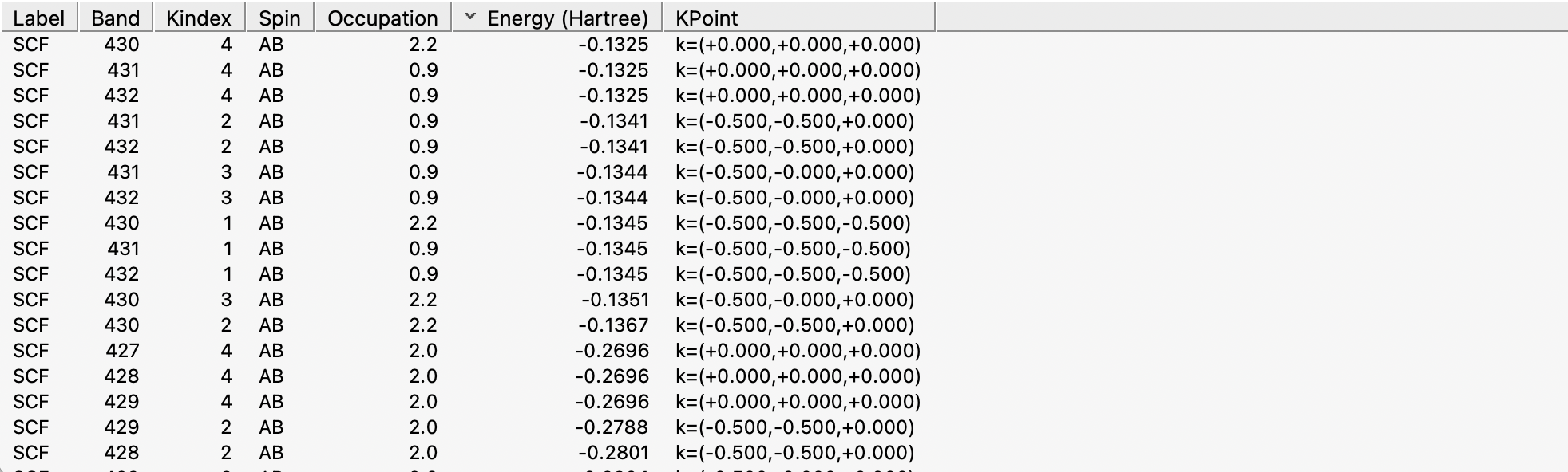
We can see that the highest occupied orbital is indeed around -0.13 Hartree and is likely corresponding to the defect. Click on it and AMSview will calculate the planar averaged.

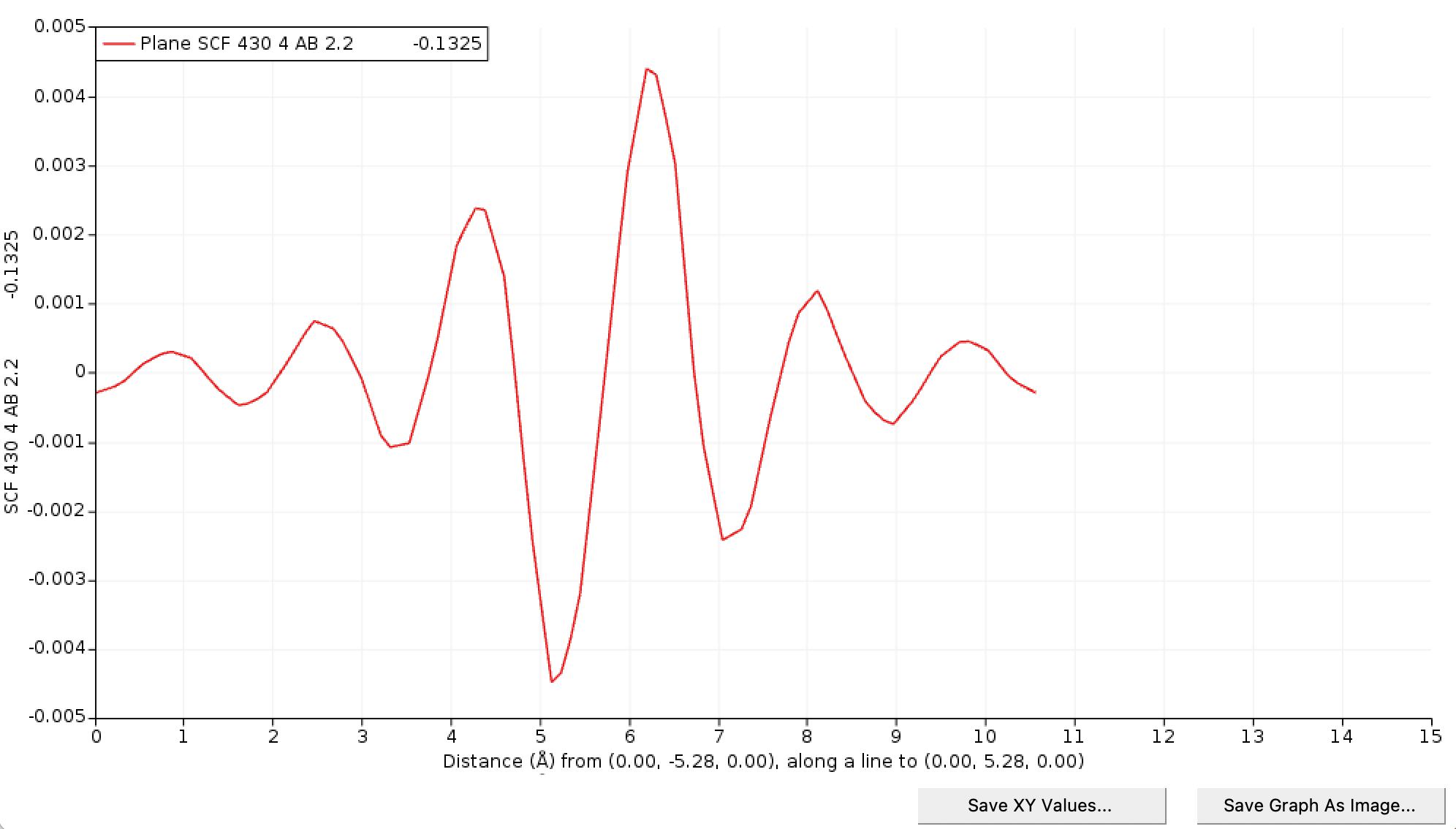
Save the graph as XY Values and name it C_diamond_3x3x3_q_HOMO.xy. Download this Python script and execute it in the same directory of the XY file you just saved.

Now we know the shape of the defect, we can solve Poisson to get the potential and the energy correction. Download this Python script that will solve Poisson. You can edit the file for your specific case. Parameters are the lattice, an energy cutoff for the basis set used in the model, the dielectric profile (here simply a scalar), the width of the Gaussian, the charge of the defect, and its location. The script will solve Poisson in 2x2x2 up to 5x5x5 supercells by defaults.

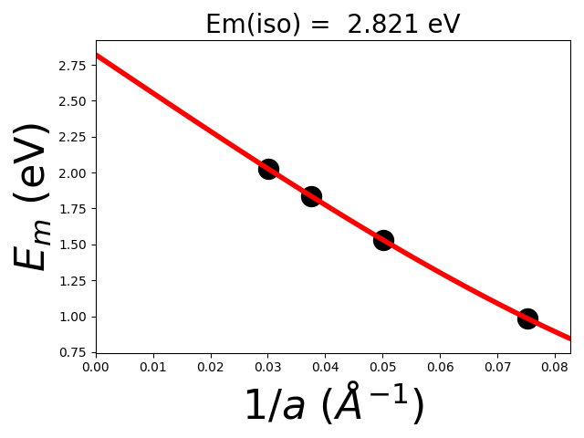
The script will output at the end the lattice correction defined above \(E_{lat} = E_{iso} - E_{per}\). Indeed, the lattice correction removes for the spurious periodic interaction in the supercell \(E_{per}\) as well as adds the isolated defect energy \(E_{iso}\) (extrapolated).

>>> 2x2x2 E_latt = E_iso - E_per =  2.821 -  0.985 =  1.836 eV
>>> 3x3x3 E_latt = E_iso - E_per =  2.821 -  1.530 =  1.291 eV
>>> 4x4x4 E_latt = E_iso - E_per =  2.821 -  1.835 =  0.986 eV
>>> 5x5x5 E_latt = E_iso - E_per =  2.821 -  2.026 =  0.795 eV

The script will also generate the potentials corresponding to each model defective cells as V_X_r.txt files. We can therefore compare the potential of the model defect to that of the DFT calculation (taken as the difference between the charged and neutral defect). This this can be used to get the validation plot below.

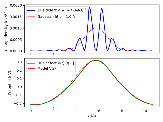
The potential difference between the model and DFT gives us access to the last term in the charged defect formation energy \(\Delta V_{q/0}\). To summarize, we have the following.

\[E^f_q = E_q - E_p + E_\text{corr} - \sum_i n_i\mu_i + q[\epsilon_F + \Delta V_{0/p}]\]

Table 7 Summary of the total energies computed with LDA for C (all in eV).

Cells	C (p)	C (0)	C (q)	\(ΔV_{0/p}\)	\(E_{latt}\)	\(ΔV_{q/0}\)	\(E^f_q corr.\)
2x2x2 (eV)	-627.68	-609.58	-620.57	-0.097	1.84	0.0	13.33
3x3x3 (eV)	-2118.32	-2099.94	-2110.44	-0.037	1.29	0.0	13.45
4x4x4 (eV)	-5021.28	-5002.84	-5013.03	-0.005	0.99	0.0	13.44
5x5x5 (eV)	-9807.05	-9788.61	-9798.59	-0.011	0.80	0.0	13.47

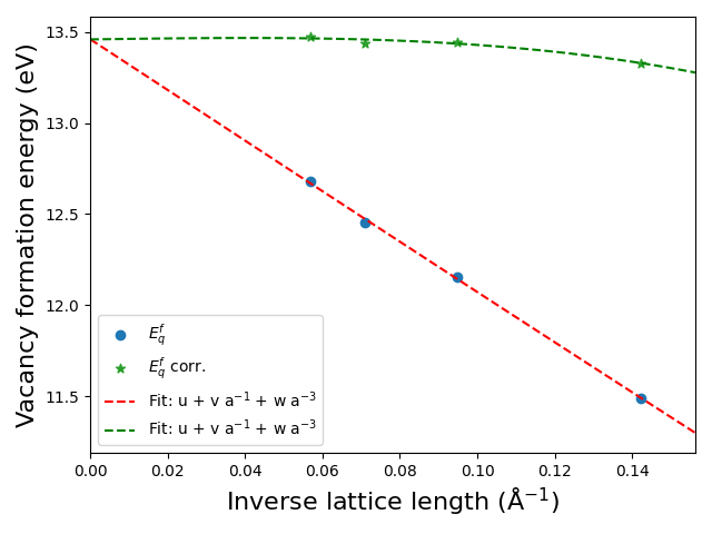
With the smallest supercell 2x2x2 we only do an error of 0.1 eV while the 3x3x3 gives an error of 0.01 eV with respect to the large 5x5x5 supercell.

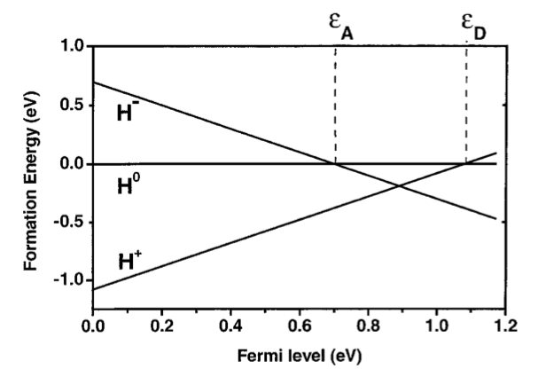
The formation energies of charged defects depend on the Fermi level, which is the reservoir with which the impurity exchanges electrons. The Fermi-level position (traditionally taken with respect to the valence band maximum) for which +1 and neutral states have equal energies defines the +/0 transition level, that is, the donor level \(\epsilon_D\); similarly, the acceptor level \(\epsilon_A\) (i.e., the 0/- transition) is defined as the point where neutral and -1 states have equal energy 3 .

Finally, 1D and 2D charged defect systems can also be corrected, as described in these papers 4 5 .

References

1

Freysoldt C, Neugebauer J, Van de Walle CG. Fully ab initio finite-size corrections for charged-defect supercell calculations. Physical review letters 102.1 (2009): 016402

2(1,2,3,4)

Komsa HP, Rantala TT, Pasquarello A. Finite-size supercell correction schemes for charged defect calculations. Physical Review B 86.4 (2012): 045112

3(1,2)

Herring C, Johnson NM, Van de Walle CG. Energy levels of isolated interstitial hydrogen in silicon. Physical Review B 64.12 (2001): 125209

4

Naik MH, Jain M. CoFFEE: corrections for formation energy and eigenvalues for charged defect simulations. Computer Physics Communications 226 (2018): 114-126

5

Github CoFFEE package

Challenges in computing charged defects