Tribology: Friction and Lubrication of Hematite

ReaxFF Tribology Friction Boundary lubrication Molecular dynamics NEMD

This tutorial will teach you how to:

• build a lubricated contact from a hydroxylated hematite slab,

• prepare a hexadecane/stearic acid mixture between two surfaces,

• equilibrate the contact under a normal load,

• perform a non-equilibrium molecular dynamics (NEMD) sliding simulation, and

• estimate an apparent friction coefficient from the tangential and normal reaction forces.

Note: The hands-on calculation is deliberately small and short so that the complete workflow can be explored on a laptop. It is intended to teach the setup. Recommended settings and results for higher accuracy simulations will be shown at the end.

Introduction

Boundary lubrication occurs when two solid surfaces are separated by a molecular film whose structure and interaction with the surfaces control the shear response. Long-chain hydrocarbons can reduce direct solid-solid contact, while polar organic friction modifiers such as stearic acid can interact more strongly with an oxide surface.

In a tribology NEMD calculation, a normal load presses the two surfaces together and one surface is driven laterally. The resulting tangential and normal reaction forces can be used to estimate friction. Here the upper hematite slab slides along the y direction while it remains free to respond to the applied load along z.

The complete workflow uses the following sequence:

• pre-optimize the hydroxylated hematite slab,

• build two opposing surfaces and insert the lubricant,

• pre-optimize the complete interface,

• equilibrate under the normal load without sliding, and

• start the NEMD run from the equilibrated coordinates and velocities.

The GUI calculation below showcases this workflow for a single mixture at a fixed normal load. The final section will show results for varying stearic acid concentrations and normal loads, obtained using higher-accuracy settings.

Prepare the Hydroxylated Hematite Slab

The starting structure of the slab was prepared beforehand starting from an α-Fe₂O₃ (0001) surface. It contains 72 atoms and a rectangular two-dimensional cell of approximately 5.05 × 8.75 Å. You can download the file here.

Note

See Crystals and Surfaces for instructions on building these surface models yourself.

We start by importing the surface structure:

1. Open AMSinput: SCM → New Input

2. Choose File → Import Coordinates (System) and select Fe2O3_0001_H2O_rectangular.xyz

Before building the contact, perform a short ReaxFF optimization of the small slab. This removes any residual strain in the geometric model.

1. Switch to the ReaxFF engine: →

2. Set Force field to FeOCHCl-ox.ff

3. Set Task to Geometry Optimization

4. Go to Details → Geometry Optimization

5. Set Optimize lattice to Yes

6. Go to Model → Geometry Constraints and PES Scan

7. Constrain the cell to remain rectangular by checking the XY component of the Freeze Strain matrix

8. Save the job using File → Save as with the name hematite_slab_relax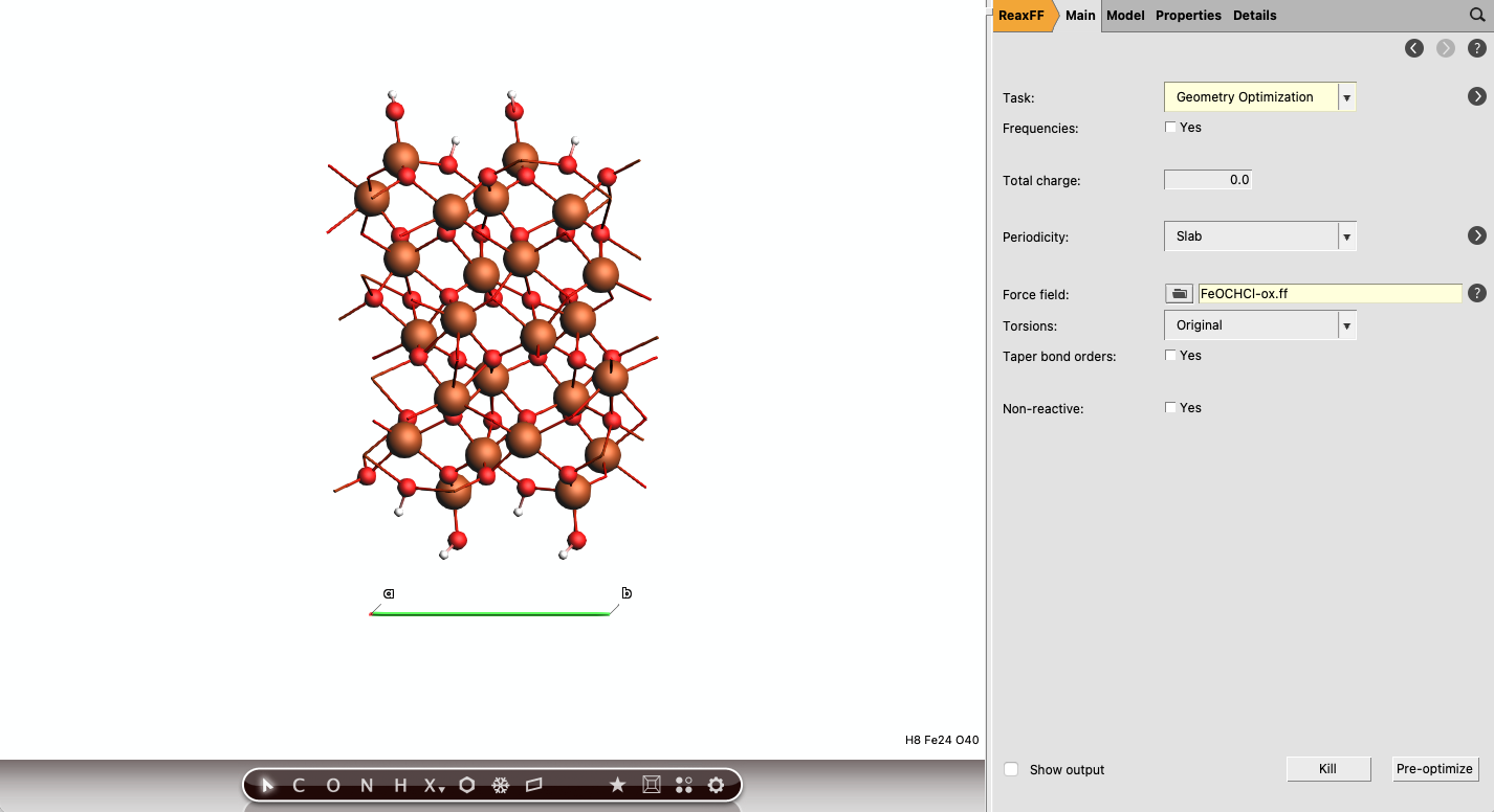

9. Start the job using File → Run

10. Choose Update Molecule once the calculation is finished to load the optimized coordinates

Fig. 39 Hydroxylated hematite slab after geometry optimization.

Build the Lubricated Contact

We increase the surface area of our slab in order to improve the resolution of the applied forces. In order to keep the present simulations short, we will use a 2 × 2 supercell as our surface model.

1. Choose Edit → Crystal → Generate Super Cell

2. Repeat the slab 2 times along the first lattice vector and 2 times along the second

We duplicate the slab in order to create the lubricant channel:

1. Use Select → Select All to select all atoms in the slab. Use Edit → Copy and Edit → Paste to duplicate the slab.

2. Choose Edit → Tune Geometry. In Translate atoms, direction, set Step to 56 and z to 1, then apply the translation by clicking the small triangle pointing to the right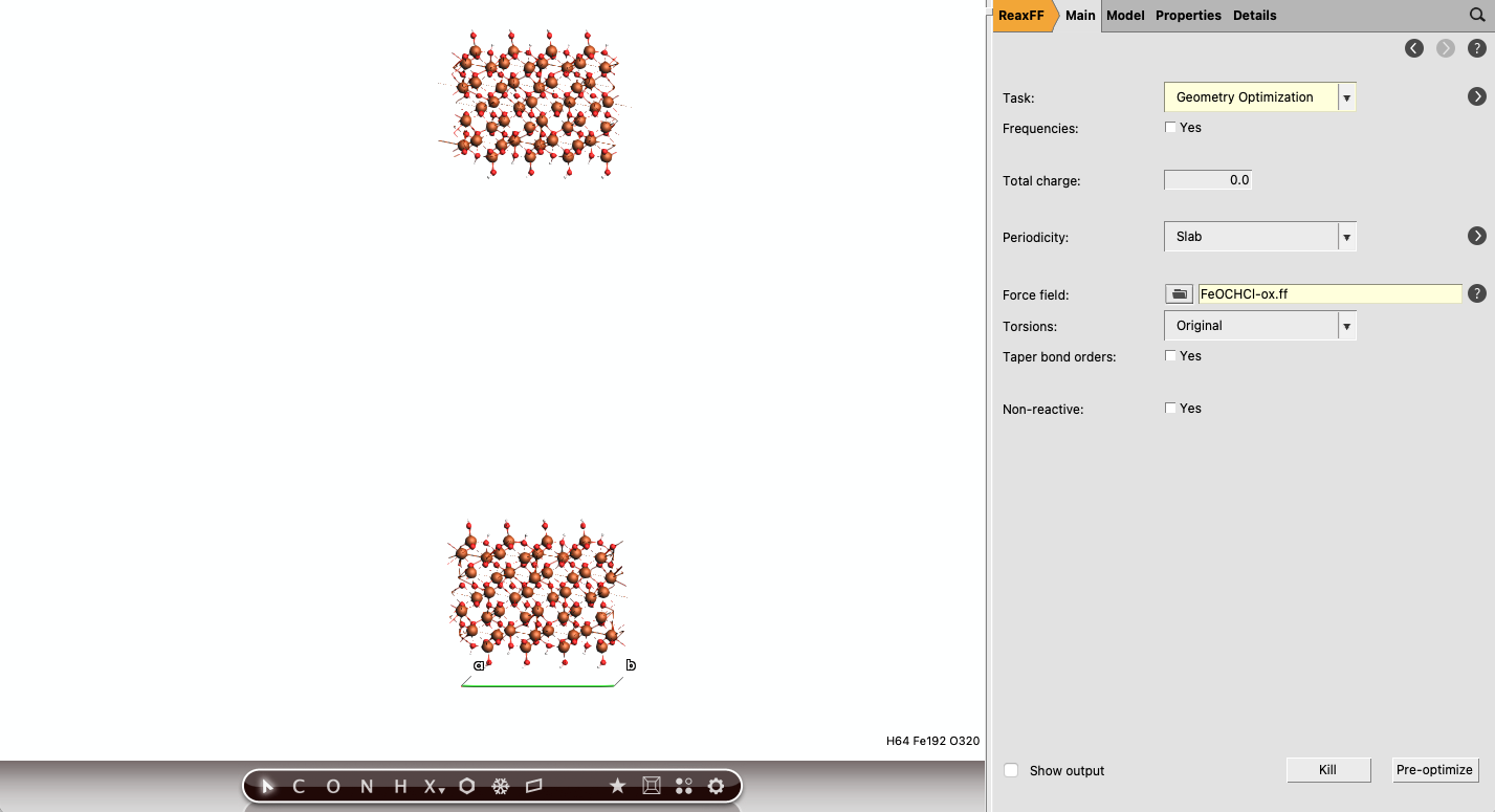

3. Wrap the atoms in the supercell with Edit → Crystal → Map Atoms To (0..1)

Fig. 40 Two opposing hematite slabs separated by an (approximately) 40 Å gap.

In order to set up the tribology simulation, the atoms will be assigned to different regions. The bottom layer of the lower slab will be frozen in place, acting as a fixed substrate for the rest of the system. The rest of the system will be subject to the MD thermostat. An additional region is defined for the upper slab, as this will be subject to the normal load.

1. Go to Model → Coordinates to view the full list of atoms. Sort the coordinates by height by clicking on the arrow icon next to the Z(A) header in the coordinates table. We will freeze the atoms in the bottom 25% of the lower slab, which should correspond to the 72 bottom-most atoms. Selecting the rows in the table will highlight the atoms in the model.

2. While the rows are selected, go to Model → Regions and click the button to create a new region. Change the name of this region to frozen

3. Use Select → Select Region → frozen and Select → Invert Selection to select the remaining atoms. Click the button to create a new region. Change the name of this region to thermo

4. Select one of the atoms in the upper slab. Use Select → Select Molecule to highlight all atoms in the upper slab. Click the button to create a new region. Change the name of this region to top_drive

Note

The overlap between thermo and top_drive is intentional: every atom in the upper slab belongs to both regions. AMS automatically excludes the net velocity imposed by Apply velocity from thermostatting, so the thermostat acts on the thermal motion of the driven slab rather than opposing its prescribed sliding motion.

This simplified scheme thermostats all mobile solid atoms, including those at the contact. It should therefore be applied consistently to every formulation being compared, because changing the thermostatted region can affect the measured friction response.

Warning

frozen must not overlap thermo or top_drive. Only the overlap between thermo and top_drive is intended.

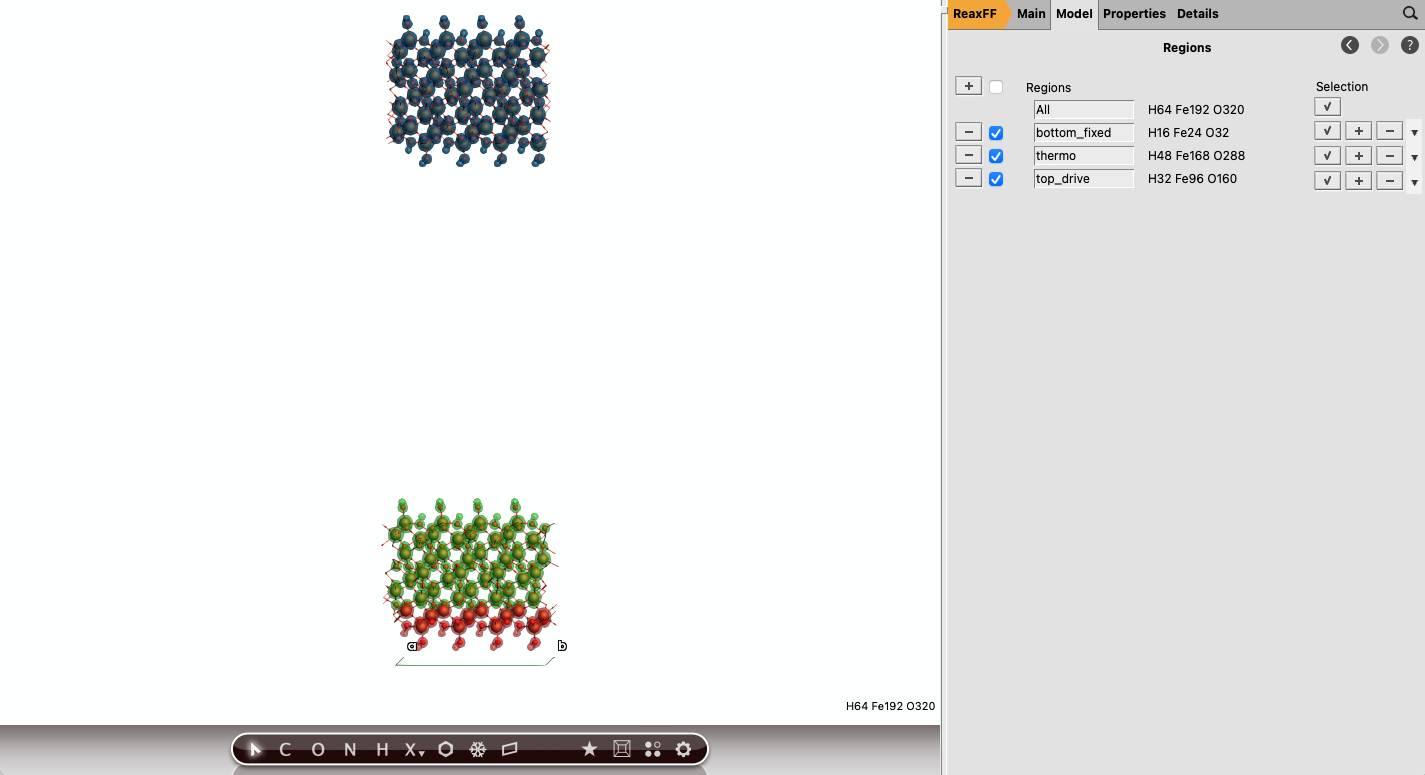
Fig. 41 Three-region assignment for the two hematite slabs. The upper slab belongs to both thermo and top_drive.

The next step is to add the hexadecane/stearic acid lubricant. An 80:20 mixture will be used here:

1. Open Builders → Packed Molecules

2. Set the height of the packing box to 76 Angstrom

3. Select Use number of molecules

4. Enter the hexadecane SMILES code CCCCCCCCCCCCCCCC as the first component. Set the number of molecules to 8

5. Use the button to add a second component. Enter the stearic acid SMILES code CCCCCCCCCCCCCCCCCC(=O)O and set the number of molecules to 2

6. Select Generate Molecules to add the lubricant

7. Go to Model → Regions. A new region has automatically been created by the packer. Change the name of the Builder region to fluid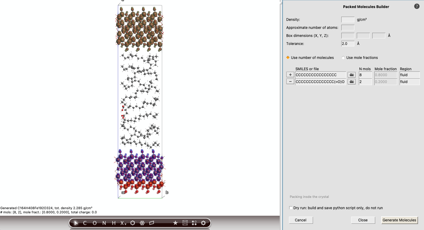

Fig. 42 Eight hexadecane molecules and two stearic acid molecules between the hematite surfaces.

The builder has created a packing of rigid molecules. To obtain a more realistic structure, we need to perform a short relaxation for the lubricant phase.

1. In Details → Geometry Optimization, uncheck Optimize lattice

2. Set the Gradient convergence to 0.05 eV/Å

3. Set the Energy convergence to 0.0001 eV

4. Go to Model → Geometry Constraints and PES Scan. Select the substrate with Select → Select Region → frozen and enable the frozen (fixed position) constraint

5. Save the job using File → Save as with the name optimize_fluid

6. Start the simulation using File → Run

7. Choose Update Molecule once the calculation is finished to load the optimized coordinates

Equilibrate Under the Normal Load

The lubricant should first equilibrate under the normal load without sliding. This allows the film thickness and normal reaction to settle before shear is introduced.

1. Change Task to Molecular Dynamics

2. In Model → MD, set Number of steps to 40000 (10 ps simulation)

3. Set Initial temperature to 300 K

4. Go to Model → MD… → Thermostat and add a new thermostat using the button

5. Set the Thermostat Type to NHC

6. Set the Temperature to 300 K

7. Set the Damping constant to 100 fs

8. Set the Atoms in Region to thermo

9. Go to Model → MD… → NEMD Velocities and Forces and click the button next to Apply force

10. Set the Force to 0.0 0.0 -3e-9 N

11. Set the Region to top_drive

12. Save the job using File → Save as with the name static_load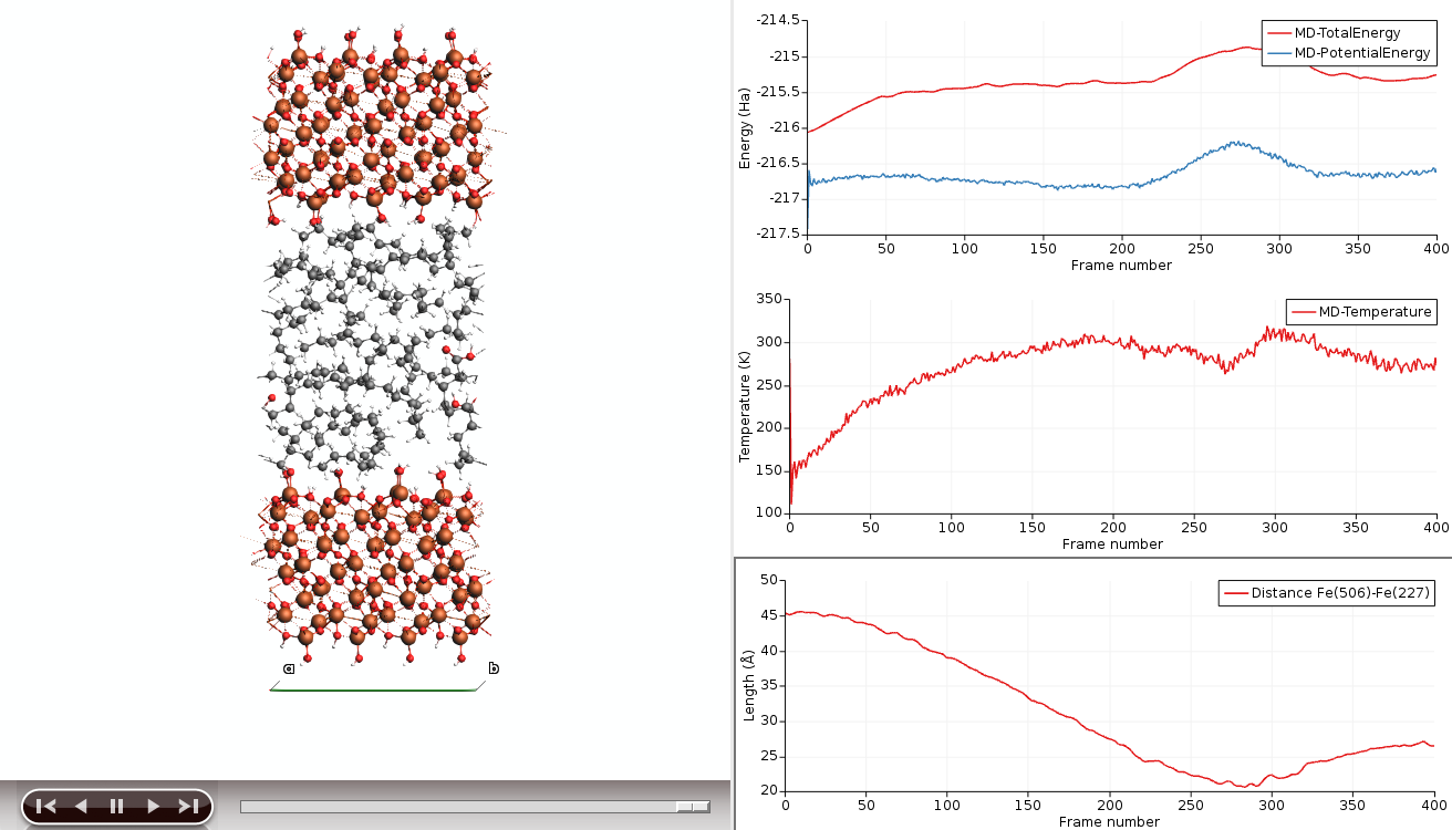

13. Start the job using File → Run

Fig. 43 Energy, temperature, and inter-slab distance during the equilibration run.

Run the Sliding NEMD Calculation

The NEMD stage starts from the static_load equilibrated coordinates and velocities, keeps the same normal load, and imposes a lateral velocity on top_drive.

1. When static_load finishes, update the coordinates in AMSinput

2. In Model → MD, set Initial velocities to From File and select the ams.rkf file from static_load calculation

3. In Model → MD, set Number of steps to 100000 (25 ps simulation)

4. Go to Model → MD… → NEMD Velocities and Forces and click the button next to Apply velocity

5. Set Velocity to 0.0 0.001 0.0 Angstrom/fs

6. Set Components to XY

7. Set Region to top_drive

8. Save the job using File → Save as with the name nemd_slide

9. Start the job using File → Run

Only the net x and y velocity components of the upper slab are controlled. The upper slab can therefore still move along z in response to the normal force. Although the upper slab also belongs to thermo, AMS excludes the imposed net velocity from the thermostat.

Note

0.001 Angstrom/fs corresponds to 100 m/s, much faster than a macroscopic sliding experiment. High velocities are commonly used in atomistic NEMD because accessible simulation times are short. The resulting friction should be interpreted for the simulated conditions.

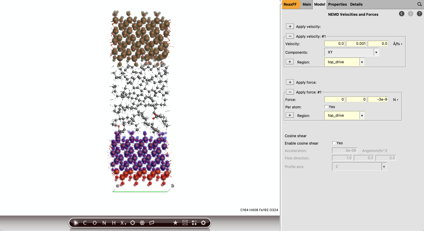
Fig. 44 Normal-force and sliding-velocity settings for the NEMD calculation.

Inspect the Forces and Estimate Friction

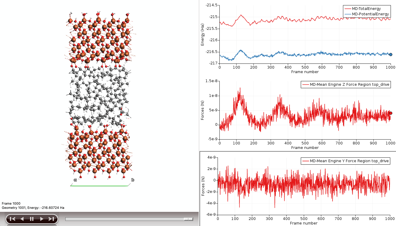
When Apply velocity is active, AMS automatically writes the instantaneous, mean, and standard deviation of the net engine force on the driven region to the trajectory. These quantities exclude the externally applied force. The tangential component opposes sliding, while the z component provides the normal reaction used in the apparent friction ratio.

To inspect the tangential and normal reaction forces:

1. Open nemd_slide with SCM → Movie

2. In AMSmovie, choose Graph → Add Graph

3. Select, MD Properties → Mean Engine Y Force Region top_drive to view the tangential force

4. Select, MD Properties → Mean Engine Z Force Region top_drive to view the normal force. After equilibration, its magnitude should be close to the applied 3 nN load

The apparent friction coefficient can be calculated from the ratio of these forces. Averaging over the second half of the trajectory (corresponding to the steady state regime) gives \(\langle F_y \rangle = -0.624454\ \mathrm{nN}\) and \(\langle F_z \rangle = 3.10325\ \mathrm{nN}\). Therefore,

\[\mu_{\mathrm{app}} = \frac{|\langle F_y \rangle|}{|\langle F_z \rangle|} = \frac{0.624454}{3.10325} = 0.201\]

The result of this example calculation produces the same order of magnitude for the friction coefficient as compared to experiment. For accurate quantitative predictions however, we need to improve the sampling settings to better account for the noisy force signals.

Fig. 45 Tangential and normal reaction-force traces for the driven upper slab.

Improving the Statistics

An increased surface area and longer simulation times can be used to increase the spatial and statistical sampling. To converge on the approximate friction coefficient:

• increase the surface area to approximately 20 × 35 Å (the load will be increased to 12.5 nN to maintain the same pressure),

• increase the duration of the NEMD run to 1 ns,

• use at least two independent replicas (trajectories) per load.

Note

These settings are recommended for research-quality simulations. The simulations can take several hours to complete, so it is recommended to run jobs on a compute cluster. It is not necessary to run these calculations to understand the workflow, so you can skip directly to the results if you want.

Tip

Re-configuring the settings for each step in the workflow can be quite laborious. A PLAMS script has been created to automatically handle the setup and analysis for this tutorial.

To start, we construct a new interface:

1. Open the optimize_fluid structure in AMSinput

2. Choose Edit → Crystal → Generate Super Cell

3. Repeat the slab 2 times along the first lattice vector and 2 times along the second. The regions should be extended automatically

A new fluid phase is created in order to remove artificial symmetry from the duplicated molecules:

1. Remove the old lubricant with Select → Select Region → fluid and Atoms → Delete Atoms

2. Open Builders → Packed Molecules

3. Set the height of the packing box to 76 Angstrom

4. Select Use number of molecules

5. Enter the hexadecane SMILES code CCCCCCCCCCCCCCCC as the first component. Set the number of molecules to 32

6. Use the button to add a second component. Enter the stearic acid SMILES code CCCCCCCCCCCCCCCCCC(=O)O and set the number of molecules to 8

7. Select Generate Molecules to add the lubricant

8. Go to Model → Regions and change the name of the Builder region back to fluid

9. Save the job using File → Save as with the name reoptimize_fluid

10. Start the simulation using File → Run

11. Choose Update Molecule once the calculation is finished to load the optimized coordinates

A static load calculation is performed on the extended system. The simulation time is increased to 100 ps in order to allow for relaxation closer to the equilibrium. This reduces noise propagation during the sliding NEMD stage. Because the surface area has increased by a factor 4, we also increase the applied normal force in order to maintain the same pressure.

1. Change Task to Molecular Dynamics

2. In Model → MD, set Number of steps to 400000 (100 ps simulation)

3. Set Initial temperature to 300 K

4. Go to Model → MD… → Thermostat and add a new thermostat using the button

5. Set the Thermostat Type to NHC

6. Set the Temperature to 300 K

7. Set the Damping constant to 100 fs

8. Set the Atoms in Region to thermo

9. Go to Model → MD… → NEMD Velocities and Forces and click the button next to Apply force

10. Set the Force to 0.0 0.0 -1.25e-8 N

11. Set the Region to top_drive

12. Save the job using File → Save as with the name static_load_125

13. Start the job using File → Run

Once the equilibration has finished, we set up the final sliding NEMD simulation. The total simulation time has increased to obtain a larger number of samples when estimating the forces. A second replica is ran in parallel to reduce the simulation length for each trajectory.

1. When static_load_125 finishes, update the coordinates in AMSinput

2. In Model → MD, set Initial velocities to From File and select the ams.rkf file from static_load_125 calculation

3. In Model → MD, set Number of steps to 4000000 (1 ns simulation)

4. Go to Model → MD… → NEMD Velocities and Forces and click the button next to Apply velocity

5. Set Velocity to 0.0 0.001 0.0 Angstrom/fs

6. Set Components to XY

7. Set Region to top_drive

8. Go to Model → MD… → Replica Exchange and set Number of replicas to 2

9. Set Swap frequency to 10000000 to create decoupled trajectories

10. Save the job using File → Save as with the name nemd_slide_125

11. Start the job using File → Run

Results

The workflow described above has been used to compare three contacts: dry hydroxylated hematite (no lubricant), hematite lubricated by pure hexadecane, and hematite lubricated by a hexadecane mixture containing 25 mol% stearic acid.

In order to analyze trends in the friction coefficients, load calculations were performed at 10, 12.5 and 15 nN. By comparing load-averaged friction coefficients, we can reduce any spurious biases introduced by the residual errors of the single-load calculations.

Table 13 Mean apparent friction coefficient from the high-load calculations.

Formulation	μ at 10 / 12.5 / 15 nN	Mean apparent μ
Dry hematite	4.391 / 3.632 / 2.976	3.666
Hexadecane	0.342 / 0.402 / 0.297	0.347
Hexadecane + 25 mol% stearic acid	0.317 / 0.294 / 0.340	0.317

A large reduction in friction is observed when introducing the lubricant film. The effect of adding the stearic acid OFM is comparatively much smaller. A 20 mol% OFM concentration only lowers the mean apparent friction by about 9%. At 15 nN load, an inverse effect is even observed. The friction reduction by stearic acid can therefore be expected to be surface-mediated, thus becoming more prominent at lower shear rates.

Note

The reported values represent apparent friction coefficients for the simulated conditions, not universal material constants. In particular, nanoscale adhesion, finite contact size, confinement, sliding velocity, and surface structure can all influence the force ratio.

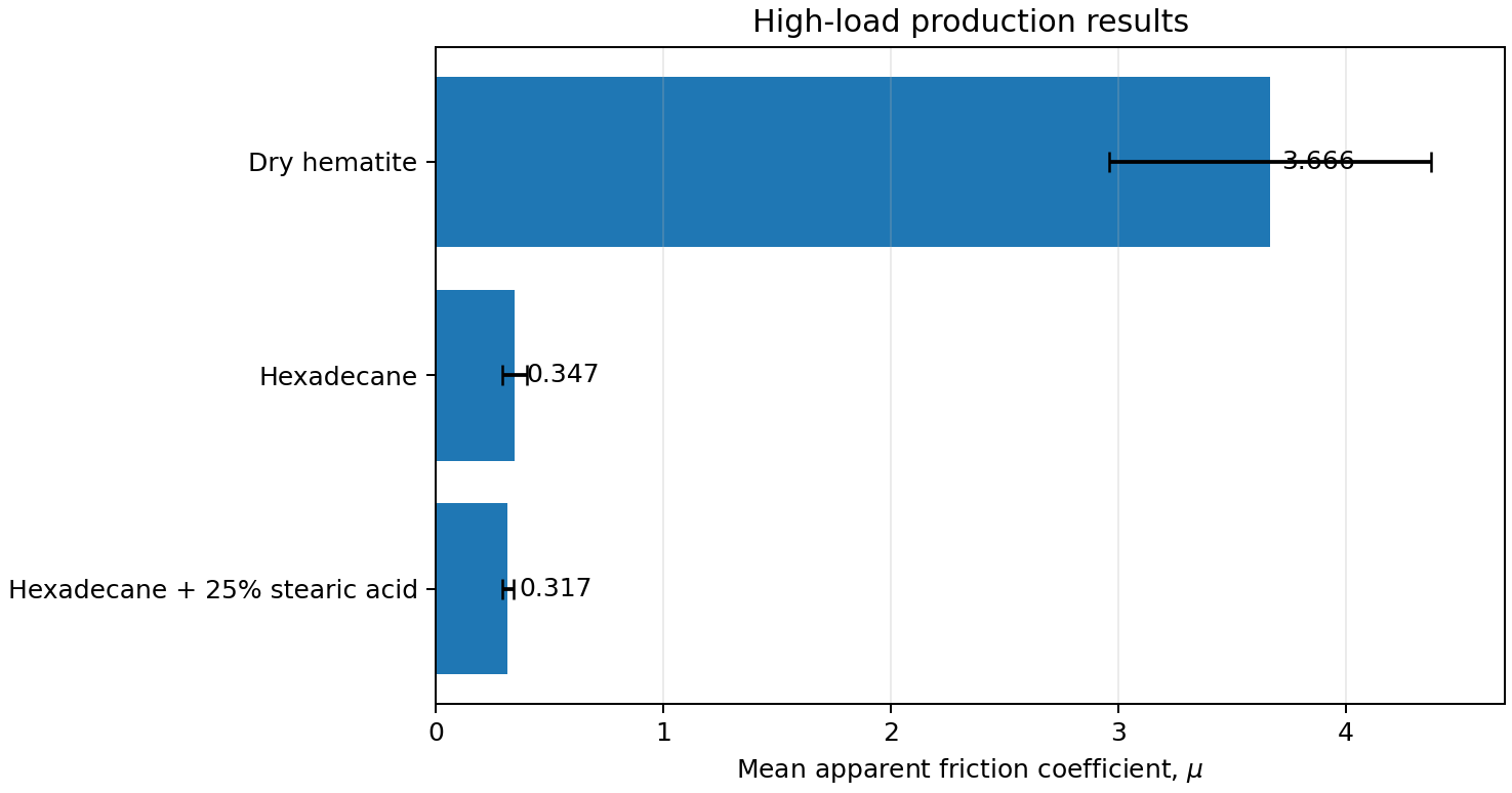
Fig. 46 Mean apparent friction coefficient for dry hematite, hexadecane, and hexadecane + 25 mol% stearic acid. The bars are averages over 10, 12.5, and 15 nN.

Summary

In this tutorial, you built a boundary-lubricated hematite contact, added a hexadecane/stearic acid film, equilibrated it under a normal load, and imposed sliding with NEMD. The workflow was applied to compare lubricant formulations.

For the systems studied here, hexadecane reduces the mean apparent friction by roughly an order of magnitude relative to dry hematite, while adding 25 mol% stearic acid gives a modest additional reduction at low load.