Acceleration

Bumblebee provides acceleration methods to enhance sampling effectiveness and reduce computation time. This tutorial will illustrate the use of these methods.

Accelerated kMC

The acceleration module is enabled by default, in order to make use of the accelerated kMC method to reduce computational cost. For this tutorial, we will compare results of accelerated and non-accelerated kMC calculations.

To start, we load the project file for the voltage sweep tutorial discussed previously (using File → Open in BBinput).

Go to the Parameters page. On the Termination tab, we set a Convergence threshold of 0.05. This will automatically stop the simulation once the current is uniform over 95% of the device. This allows us to compare the different acceleration methods at the same degree of convergence. We also do not need to manually monitor the simulations. Go to the Modules tab and make sure that the acceleration module is disabled.

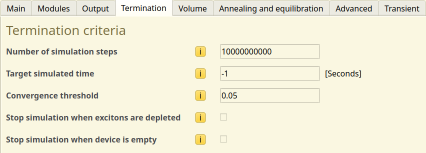
Fig. 47 Convergence settings in the parameter set

We save the updated project with a new name: File → Save As → reference.bee. This simulation will be our non-accelerated reference. Use File → Run to start the simulation.

We now switch to the Modules tab and turn on the acceleration module. The settings in the Acceleration tab will be kept at their default values. We save the project with File → Save As → acceleration.bee and start our accelerated kMC simulation using File → Run.

AMSjobs will now show 2 active simulations. Because a convergence threshold has been set, we can simply wait for the simulations to finish. We can then compare the output of the simulations in BBresults.

The JV profiles predicted by both simulations appear to be nearly identical, with any variance mostly being due to the stochastic nature of the kMC method. The accelerated calculation appears to have converged in fewer steps than the non-accelerated reference. This is seen by the lower number of datapoints in the convergence graph.

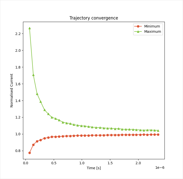
Fig. 48 Convergence of the transient current at 5 V

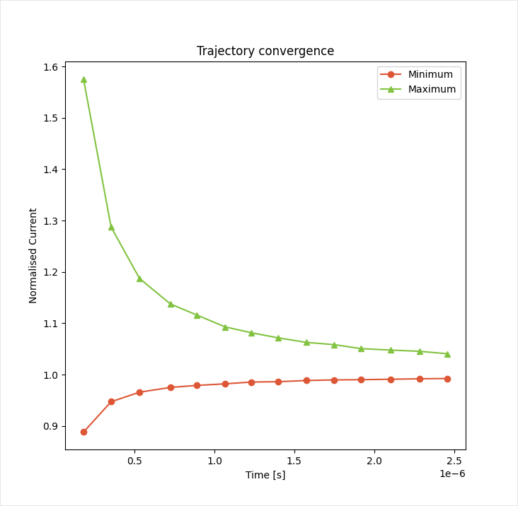
Fig. 49 Convergence of the transient current at 5 V with accelerated kMC

Comparing the exact step counts from the table (or the time_progress.out file), the accelerated kMC method required 60% fewer iterations to reach the steady state, thereby also reducing the calculation time by 60%.

Rate Booster

A rate booster is also available to promote anisotropic charge transport along the electrode current. This increases the rate at which the system equilibrates and enhances the sampling of rare events that are typically of interest to OLED performance.

The relative rates of the parallel and perpendicular transfer processes can be modified. Specifying a priority factor of 1.2 for the carrier transport will increase the parallel current sampling frequency by 20%. The simulation will then spend less time sampling diffusive off-axis transport, improving computational performance, particularly in the low-voltage regime.

We open the acceleration.bee file created in the previous step. On the Parameters page, we navigate to the Acceleration tab to find the settings for the rate booster. We modify the Parallel bulk sampling frequency to 1.2:

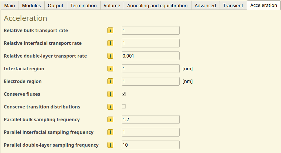
Fig. 50 Acceleration settings in the parameter set

Parameters for the double-layer interactions are determined automatically in order to match with the injection barrier of the electrodes. These parameters will be left alone for now.

We save the project with File → Save As → booster.bee and start our boosted kMC simulation using File → Run. Once the calculation has finished, we can compare the output with BBresults:

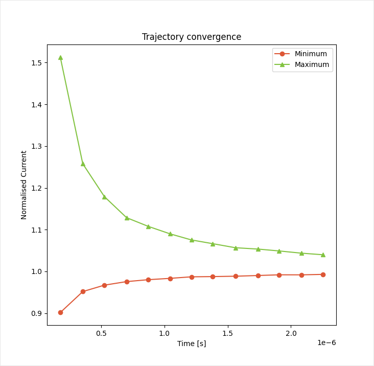
Fig. 51 Convergence of the transient current at 5 V with a rate booster enabled

Compared to the accelerated kMC method, we find that convergence is achieved in 8% fewer steps by enabling the rate booster. While this performance gain is smaller than that of the accelerated kMC method itself, these cost savings can add up when performing larger parameter screenings.

Note

The rate booster adds an anisotropic bias to the distribution of process frequencies. This bias can alter the kMC trajectories, influencing the device statistics.

Similar to the determination of the electrode transfer barrier, it is necessary to verify that the priority factor does not alter the device behavior.

A single trajectory instance can be evaluated in order to determine the correct acceleration settings. Once determined, the parameter set can be updated. Subsequent simulations can be performed at significantly reduced cost.

Because the rate booster module does not alter the actual opto-electronic process parameters, the same acceleration settings can be used at various currents. Care should be taken, however, that the priority factor was determine at a current where opto-electronic processes were energetically accessible.

For example: when annihilation processes are included in the simulation, you should confirm that sampling of these processes occurred in the trajectory instance that was used to determine the acceleration settings.

The necessary process event counts can be found in the Sweep → Profiles section of BBresults.

Configuring Output

Writing output to the file system can become a bottleneck for the kMC simulation, as write speeds are typically slow compared to the evaluation of processes in Bumblebee.

Faster simulation times can be obtained by choosing longer output intervals. This does come with a risk that fewer checkpoints are generated to enable simulation restarts in case of job interruptions. As the average device statistics typically contain the simulation properties of interest, the reduced amount of intermediate output itself is often considered inconsequential.

Aside from reducing the reporting interval, the content of the simulation output itself can also be reduced. The Output settings in the parameter sets allow users to disable undesired statistics from the output by de-selecting the appropriate set of files. This reduced the memory volume of the output, particularly for transient data, event logs or 3D distributions.

Cost Scaling

The cost of a Bumblebee simulation scales with the volume of the device. Modeling of devices with many layers or large surface area will require longer simulation times, simply because the carriers have to traverse longer distances and sampling has to be conducted over a larger number of gridpoints.

For devices with a large surface area, one has the choice between conducting a single large-area simulation or splitting the total surface area between multiple parallel instances. This choice typically has little effect on the overall simulation cost. Parallel distribution tends to be preferred when a larger number of cores is available, as utilization of multiple CPUs allows faster access to simulation results. The required number of CPU-hours nevertheless remains mostly unaltered.

When conducting simulations on very large stacks, the time required to equilibrate the device increases, as does the required number of samples to properly characterize the device. Since most large-stack OLED devices tend to represent multi-stack junctions, it is possible to coarse-grain the simulation by splitting up the stack. Simulations can be conducted on individual stack segments. By matching the current-voltage profiles of the segments, the behavior of the multi-junction system can be reproduced. Note however, that this is only possible when interactions between the junctions are negligible. For cases where coarse-graining is not viable, utilization of the acceleration module is recommended to improve sampling efficiency.