Advanced Initialization¶

By default, devices are initialized without charge carriers. Polaron injection is simulated at the electrode interface to model the population of the charge density distribution. For studying bulk materials, a minimum charge carrier density is specified to populate the device without direct electrode contacts.

As a result, the initial state of the device can be quite far from equilibrium. The first segment of the kMC simulation will be dominated by carrier diffusion through the device, before photonic processes are able to occur. In this tutorial, we will discuss charge carrier doping as a method for pre-initialization of device distributions.

Charge Carrier Initialization¶

An additional set of charges can be distributed throughout the device at the start of the simulation. This can be utilized to accelerate device equilibration, to simulate specific off-equilibrium conditions or to investigate dopants and trap states. Initial carrier concentrations are configured in the stack editor by specifying the fraction of sites that is occupied by a given type of polar or exciton.

Import Materials¶

In this tutorial, we will showcase how to configure dopants during the simulation of a single-layer phosphorescent OLED. We start by importing the host and guest materials.

Open BBinput from the main SCM menu (SCM → BBinput). Select the File → Import → Material option to access the material database. Use the Search search option to find the mCBP host and the Ir(dmp)3 phosphorescent emitter. Select the checkbox next to these materials and use the Import option to add the materials to the project.

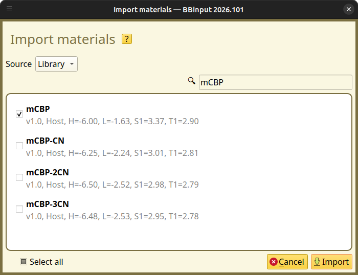
../_images/import_materials_655ff521.png — Fig. 126 Import materials from the *Materials Database* in BBinput¶

Create a Host-Guest System¶

Navigate to the Compositions page. Pure compositions for our host and guest have been created automatically. We will use the AddButton button to create a new composition for a host-guest blend.

In the composition editor, use the AddButton button in the Fractions table to add the mCBP and Ir(dmp)3 materials. We set a fraction of 0.9 for mCBP and 0.1 for Ir(dmp)3. Select Save composition to add the new blend to the project.

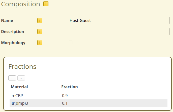
../_images/composition_08026c6c.png — Fig. 127 Host-guest blend in the composition editor¶

Create a Single-layer Device¶

Navigate to the Stack page. Use the AddButton button in the Layers table to create a single-layer OLED device. We select the host-guest mixture as the layer composition and change the thickness to 20 nm.

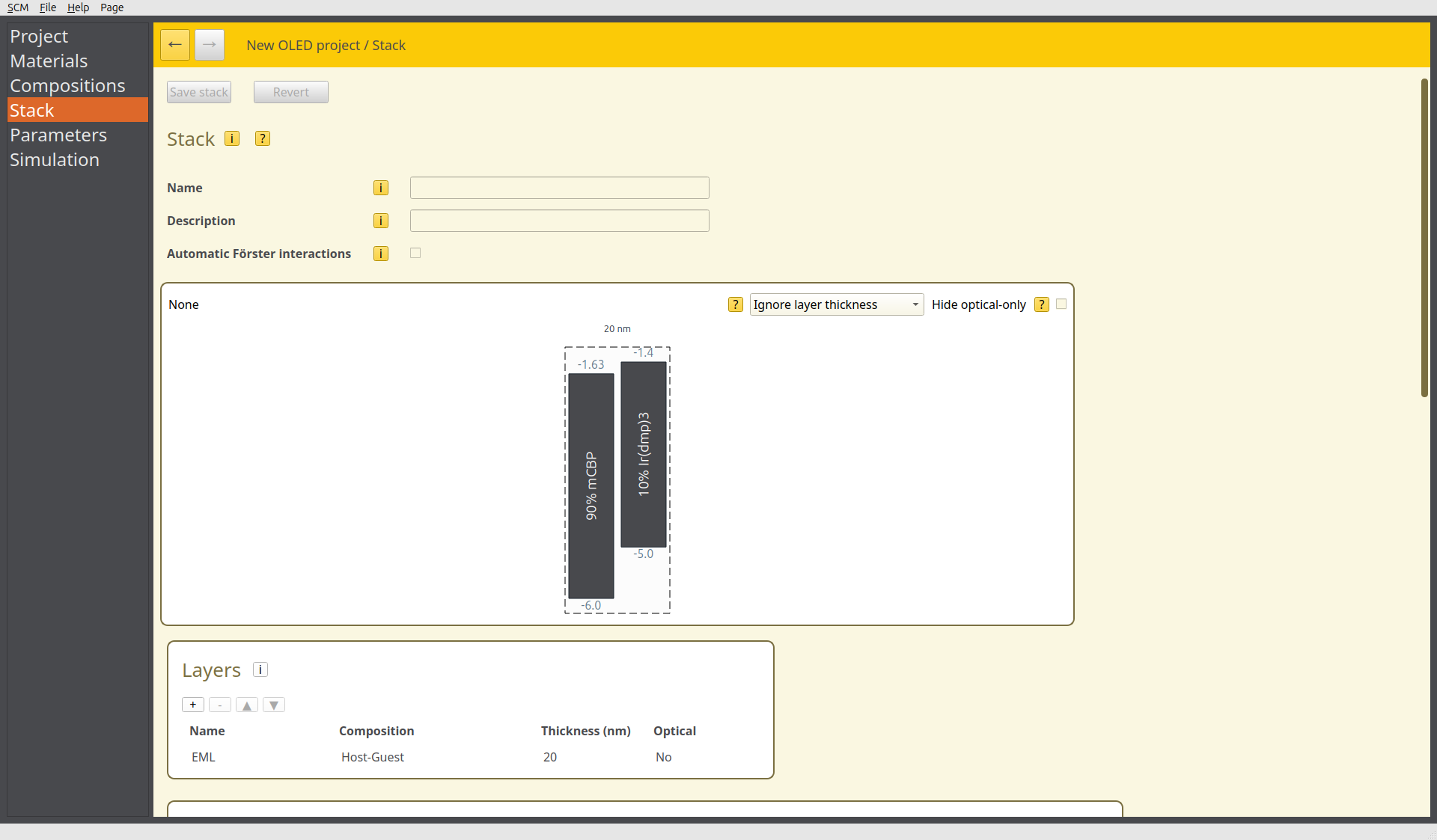
../_images/stack_808128ba.png — Fig. 128 Single-layer OLED device in the stack editor¶

Instead of starting with an empty device, we can add charges to the system by choosing dopants. We navigate to the Dopants table in the Stack page. Use the AddButton button to create 2 new dopants. Both dopants will be added to the host mCBP material. We set the type of the first dopant to Electron and the second dopant to Hole. The fraction will be set to 0.005 for both types. This sets the number of molecules that will contain charges.

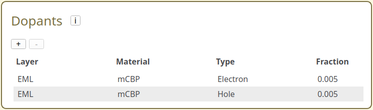
../_images/dopants_a44f36bf.png — Fig. 129 Dopant configuration in the stack editor¶

Output Settings¶

Navigate to the Parameters page. On the Output tab, we set the Report interval to 10,000 and the Output interval to 100,000. On the Termination tab, we set the Convergence threshold to 0.1. The simulation will then end automatically once the current is uniform across 90% of the device.

Starting the Simulation¶

For this example, we will perform a single voltage point calculation, which is configured by default. To reduce the resources required to run this tutorial, we navigate to the Simulation page and set both first trajectory and last trajectory to 1.

Use File → Save and File → Run to start the simulation.

Simulation Output¶

We can monitor the progress of the simulation using BBresults (SCM → BBresults). Compared to the simulation for the undoped system, charge carrier initialization enhances the rate of convergence as the initial charge carrier distribution is closer to the equilibrium.

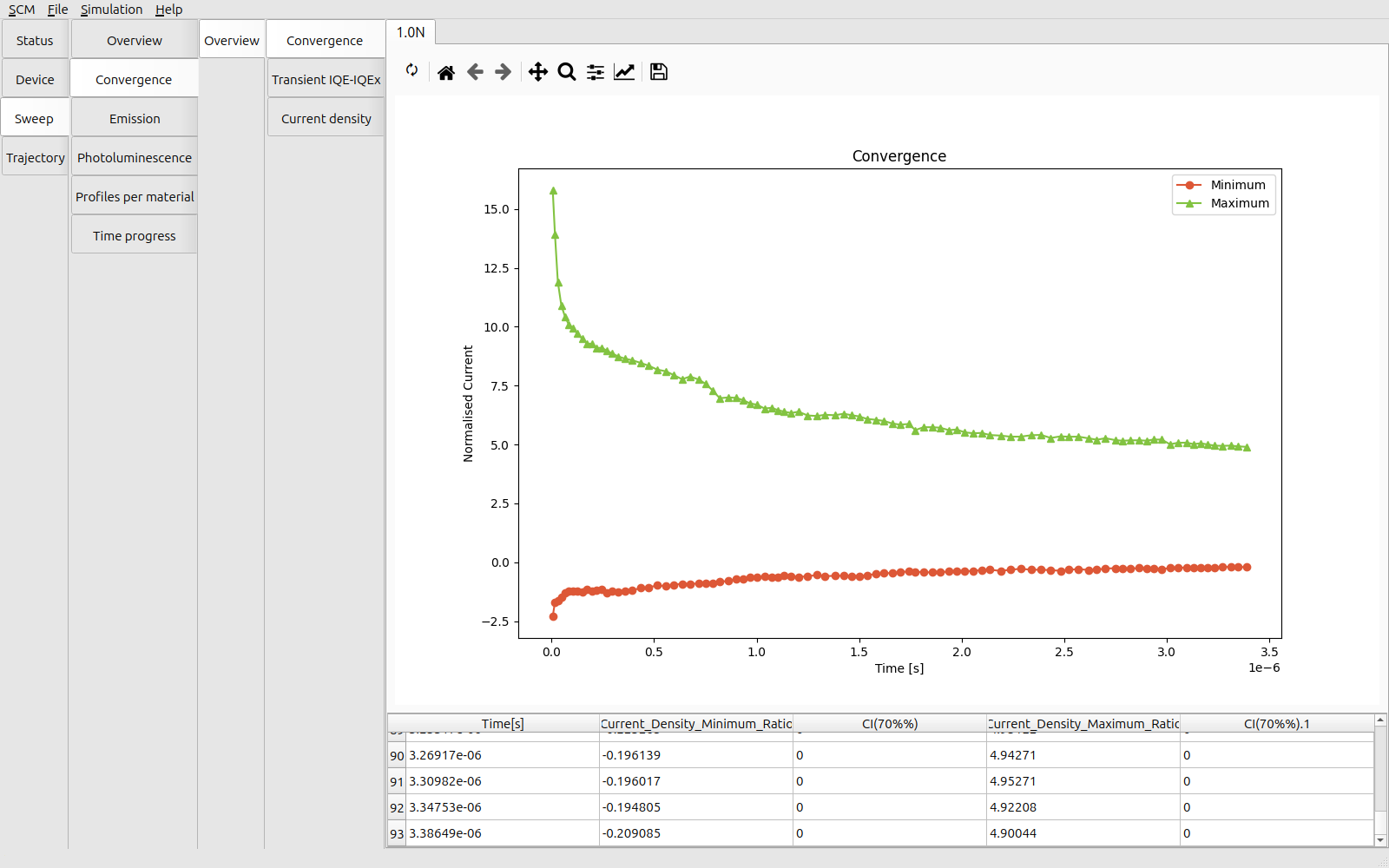
../_images/convergence_doped_8075bc9b.png — Fig. 130 Convergence of the transient current for the doped device¶

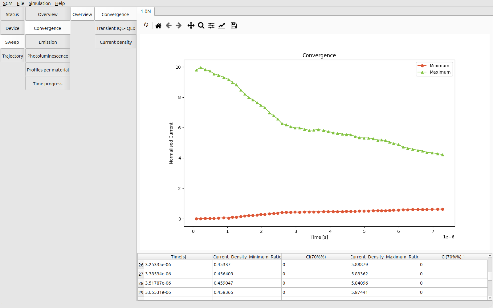
../_images/convergence_empty_c20786bf.png — Fig. 131 Convergence of the transient current for an undoped device¶

In addition, by initializing carriers inside the device, we also see that exciton generation at the emitter occurs earlier in the simulation runtime. This provides faster access to the statistics on the excitonic processes.

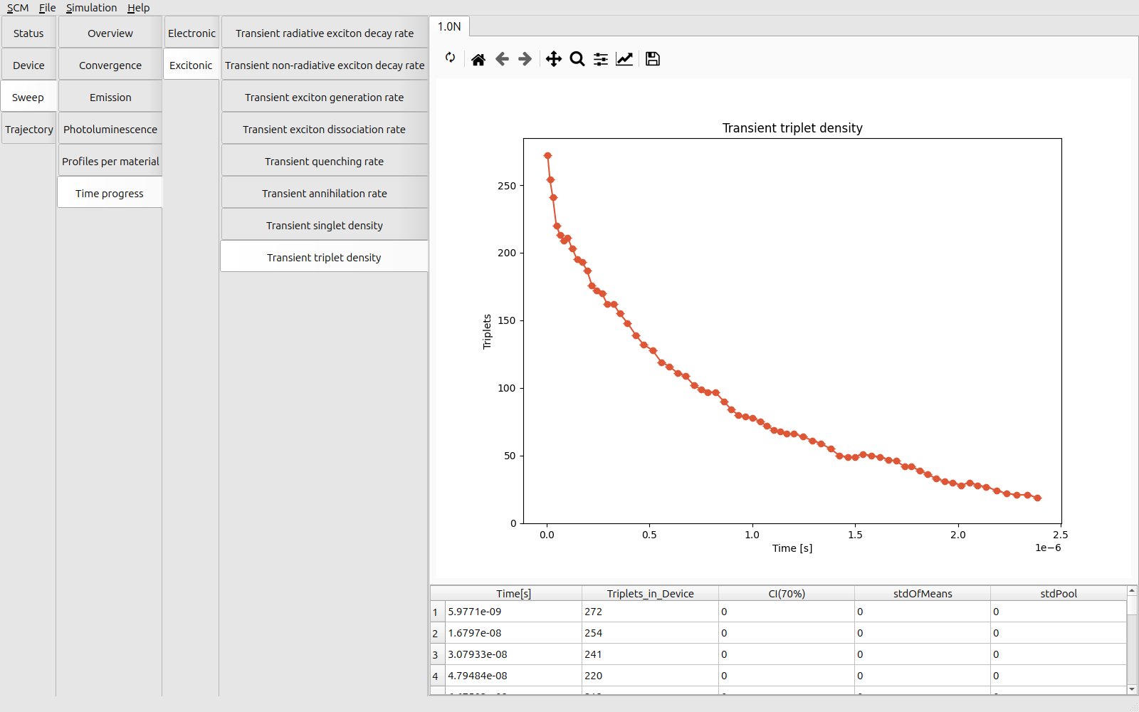
../_images/triplets_49b95dc2.png — Fig. 132 Transient exciton density inside the doped device¶

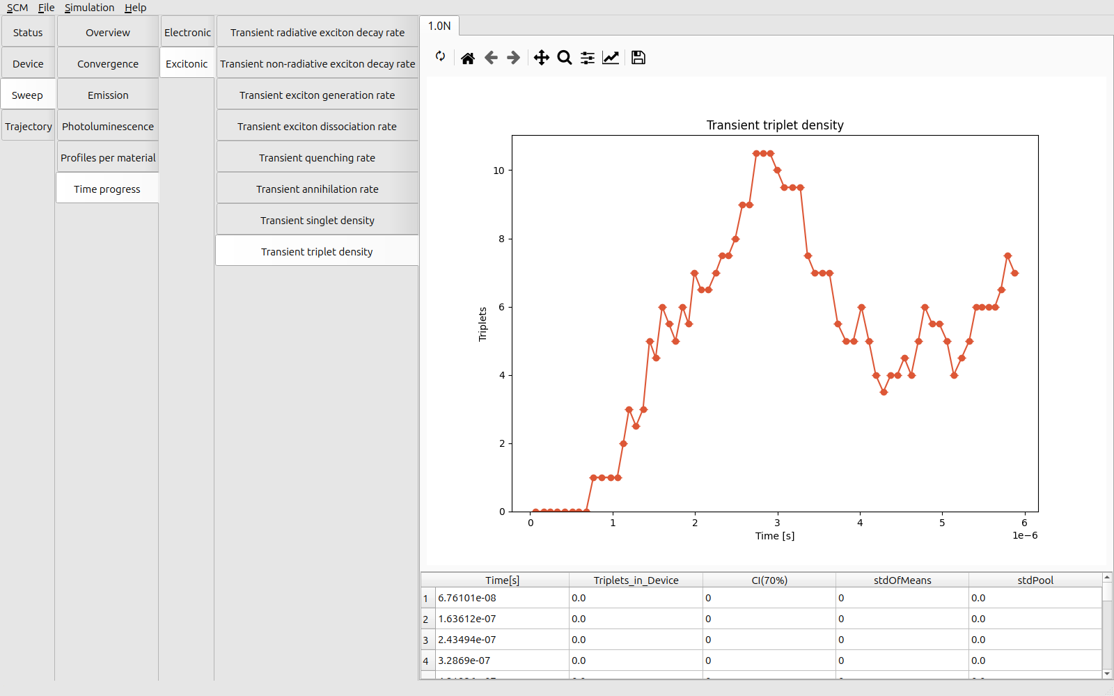
../_images/triplets_empty_da17b20f.png — Fig. 133 Transient exciton density inside the undoped device¶

Tip

To get the best performance, the initial charge carrier concentration should be as close as possible to the device equilibrium. Charge carrier distributions obtained from previous simulations can provide a suitable first estimate.

Due to differences in electron and hole mobility in the device, the optimum starting conditions may require using a different dopant fraction for electron and holes.