Layer Morphology

Composition are used to define layers containing multiple materials. This allows for the generation of host-guest systems or exciplex blends. Composites can also be used to create graded emission zones or to model the microscopic roughness of layer interfaces.

In this tutorial, we will showcase how to simulate these complex morphologies with Bumblebee.

Basic Compositions

Basic compositions were used in the preceding tutorials. These compositions assume that the materials are homogeneously distributed within a layer. The distributions are generated at the start of the simulation. When multiple trajectories are used, each instance will have its own unique distribution.

The Advanced compositions allow for the definition of gradients to specify more complex layer morphologies.

Import Materials

We will create a new project with BBinput (SCM → BBinput). To get started, we choose to import our materials from the built-in database. Select the File → Import → Material option to access the material database. Use the search option to find the CBP host, the Ir(ppy)3 emitter, the Ir(dmp)3 emitter and the TAPC transport material. Select the checkbox next to these materials and use the Import option to add the materials to the project.

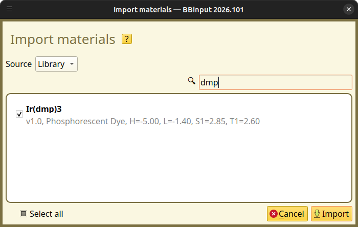
Fig. 52 Import materials from the Materials Database in BBinput

Layer Gradients

We navigate to the Compositions page. Here, we will create several Advanced compositions that can be used as the layers for our stack.

Linear Gradient

Use the button to create a new composition for a host-guest blend. This will open the composition editor. Select the Morphology option to access the advanced composition generators.

For Advanced compositions, we always start by defining the background material. The background material is used to close the material balance at each gridpoint, assuring that the fractions sum to 1. If no morphology is specified, the background material will make up the entire layer. For this example, we will select CBP.

After specifying a background material, we then get to add morphology generators. These are used to add materials to the composition. The generator type specifies the material distribution that will be obtained. Use the button in the Morphology table to add a generator. The Linear generator will be selected by default.

We will use the linear gradient generator to add an Ir(ppy)3 dye to the CBP host. The material can be changed to Ir(ppy)3 in the Morphology table. Note that when the Linear gradient is selected, a new editor will appear at the bottom of the page. This editor allows us to modify the gradient.

For the linear gradient, the material fraction is specified at the layer edges. A linear interpolation is used to determine the fractions at the interior gridpoints. For this example, we will have the gradient range from a fraction of 0.2 at the start of the layer, to a fraction of 0.8 near the end of the layer.

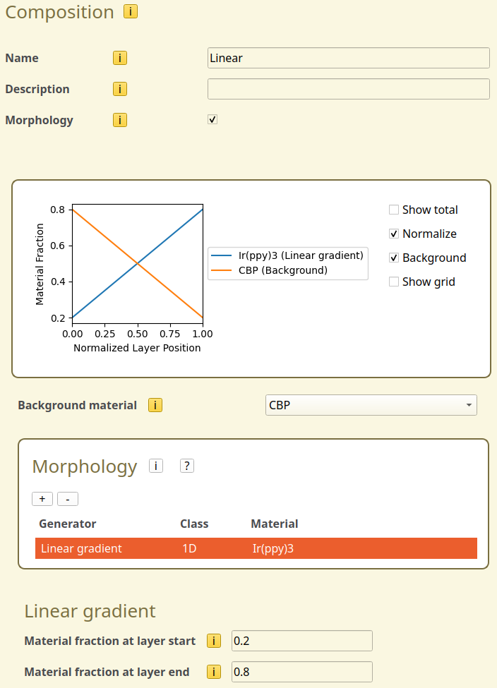
Fig. 53 Linear gradient configuration in the composition editor

Use the Save composition button to save the composition as part of the project.

After updating the gradient, the morphology view now includes a figure that previews the material distribution in the layer. We can enable the Normalize and Background options to view both components.

Trapezoid

To compare the different generators, we will create a new composition using a Trapezoid. Use the button to add a composition and select Morphology to access the advanced generators. We again set the background material to CBP and use the button in the Morphology table to add a generator. We change the generator to Trapezoid and choose Ir(ppy)3 as the material.

The trapezoid generator can be used to combine multiple linear interpolations. In order to create a trapezoidal gradient, the material fraction can be specified at various locations inside the layer. Linear interpolation is used to determine the fractions at the remaining gridpoints. The locations are specified as a fraction of the layer width. This allows the morphology to be used with different stacks. At each location, we will set the fraction of Ir(ppy)3.

In the trapezoid settings (which appear after selecting the trapezoid generator in the Morphology table), we can use the button to add points to the trapezoidal gradient. We will use a simple 3-point trapezoid for this example. The list of coordinates is given in the figure below.

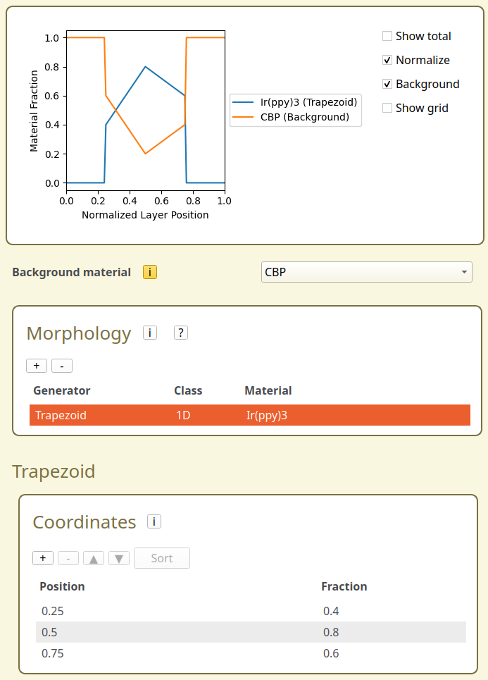
Fig. 54 Trapezoidal gradient configuration in the composition editor

If the list of coordinates does not include the edges of the layer (\(x=0,\,x=1\)), all fractions outside the trapezoid range will be set to 0. This can also be seen in the morphology preview at the top of the page.

Now that the trapezoid has been configured, use the Save composition button to save the composition as part of the project.

Exponential Gradient

We will create a new composition to illustrate the use of the exponential gradient. Use the button to add a composition and select Morphology to access the advanced generators. We again set the background material to CBP and use the button in the Morphology table to add a generator. We change the generator to Exponential and choose Ir(ppy)3 as the material.

The exponential gradient will add dye molecules according to an \(x^x\) distribution within a segment of the layer. These distributions are used to resemble imperfect deposition profiles. The start and end points of the profile are given in fractional coordinates, which allows the generator to be used for different layer thicknesses. Locations outside of the given range will have a fraction of 0.

Selecting the Exponential generator in the morphology table will make the gradient settings appear at the bottom of the page. For this example, we will set the starting coordinate to 0.2 and the final coordinate to 0.8. As seen from the morphology preview at the top of the page, the outer edges of the layer, 20% on either side, do not contain any dye.

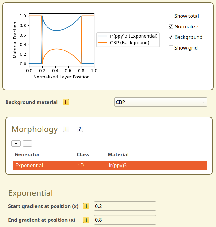
Fig. 55 Exponential gradient configuration in the composition editor

Use the Save composition button to save the composition as part of the project.

Multiple Gradients

Generators can be combined to create more complex morphologies. We will create a new composition to illustrate the use of multiple gradients.

For this example, we will consider a host-guest system containing 2 dyes: Ir(ppy)3 and Ir(dmp)3. Use the button to add a composition and select Morphology to access the advanced generators. CBP is used as the host material and is therefore set as the background material. We will use a Linear generator to create a static Ir(dmp)3 fraction of 0.1. The Trapezoid is used to add an Ir(ppy)3 gradient at the edges. The Exponential gradient is used to add a dense Ir(ppy)3 region to the center of the layer.

Use the button to add the 3 generators to the Morphology table. The required settings for each of the generators are detailed below.

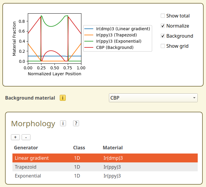
Fig. 56 Morphology configuration for multiple gradients in a dual-dye system

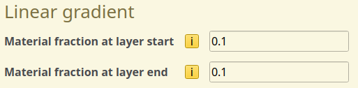
Fig. 57 Linear gradient configuration in the dual-dye system

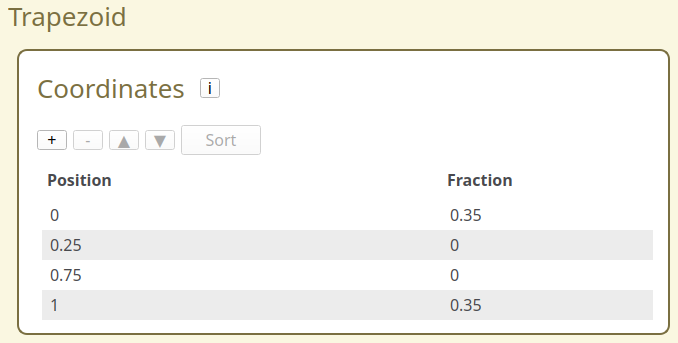
Fig. 58 Trapezoid configuration in the dual-dye system

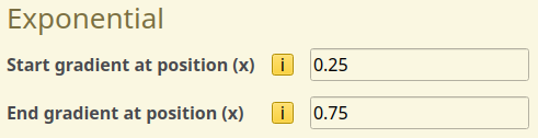
Fig. 59 Exponential gradient configuration in the dual-dye system

We use the Save composition button to save the composition as part of the project.

Create Projects

At the end of these steps, you should now have 4 advanced compositions. We will configure a simple simulation for a single-layer device to showcase the differences between their morphologies.

Navigate to the Stack page and use the button on the Layers table. This will create our single-layer stack. We update the layer thickness to 50 nm and change the composition to use the Linear gradient created earlier.

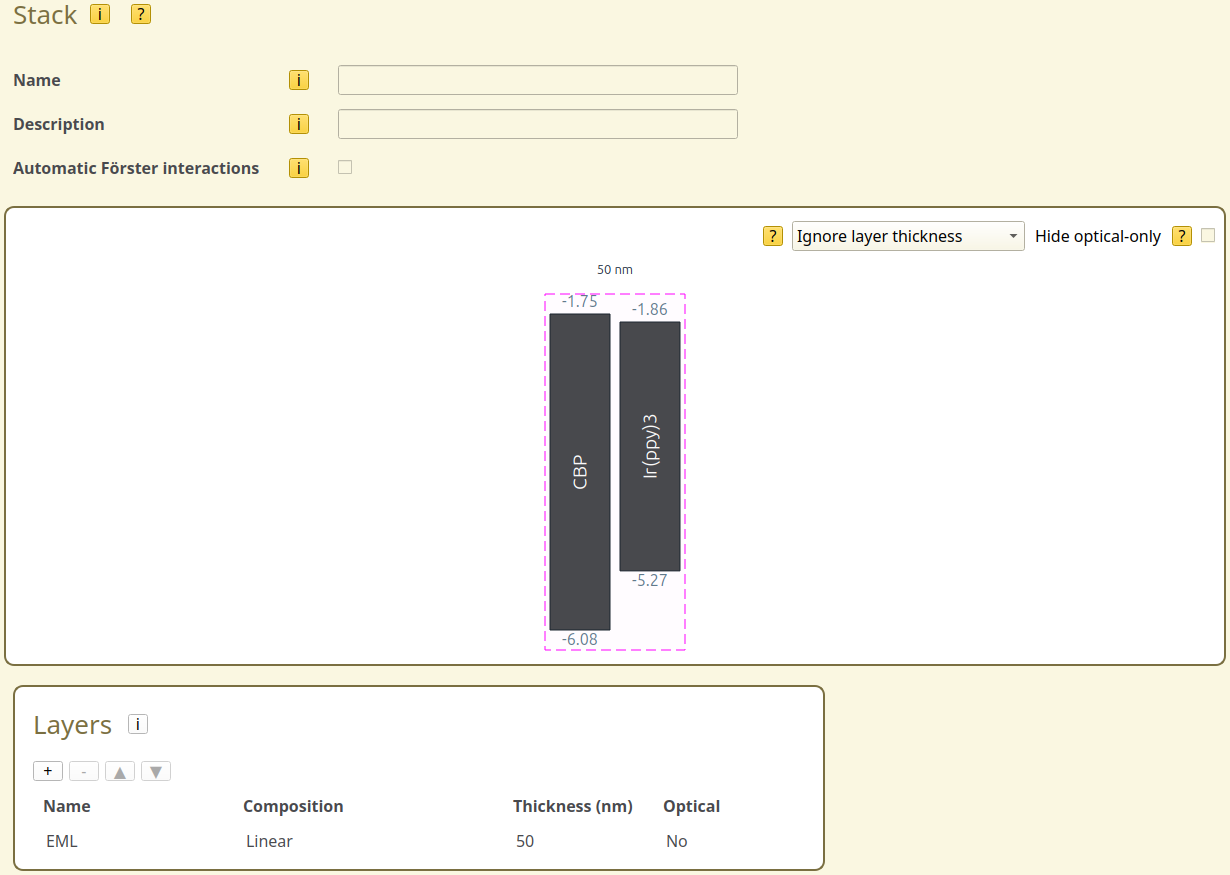
Fig. 60 Single-layer device setup in the stack editor

We then go to the Parameters page. In the Termination tab, we set the number of simulations steps to 100,000. This will run a very short simulation, which will mostly serve for us to visualize the material distributions. On the Output tab, we set the report interval to 1,000 and the output interval to 100,000 to match the shorter runtime. The remaining parameter settings will be kept at the default values.

We save the project using: File → Save As → Linear.bee

Afterwards, we can edit the stack to easily create new projects for the other compositions.

• Go back to the Stack page and replace the composition with the Trapezoid. Save this as a new project using: File → Save As → Trapezoid.bee

• Go back to the Stack page and replace the composition with the Exponential gradient. Save this as a new project using: File → Save As → Exponential.bee

• Go back to the Stack page and replace the composition with the Dual-dye system. Save this as a new project using: File → Save As → MultipleGradients.bee

Starting the Simulations

Open AMSjobs from the main SCM menu (SCM → Jobs). Separate jobs will have been created for each of the 4 projects. Select the jobs and use Job → Run to start the simulations.

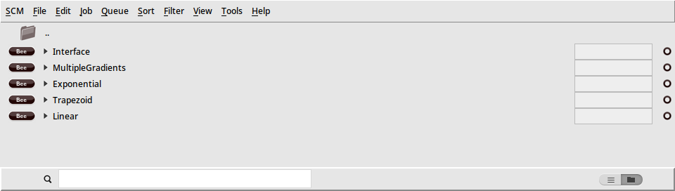
Fig. 61 List of Bumblebee simulations in AMSjobs

Visualizing Gradients

Once the simulations have started, we can view the generated morphologies with BBresults.

Select a job in AMSjobs and use SCM → BBresults to automatically load the data from the corresponding results folder. The generated morphologies will then be shown in the Trajectory → Morphology → Cross-section tab.

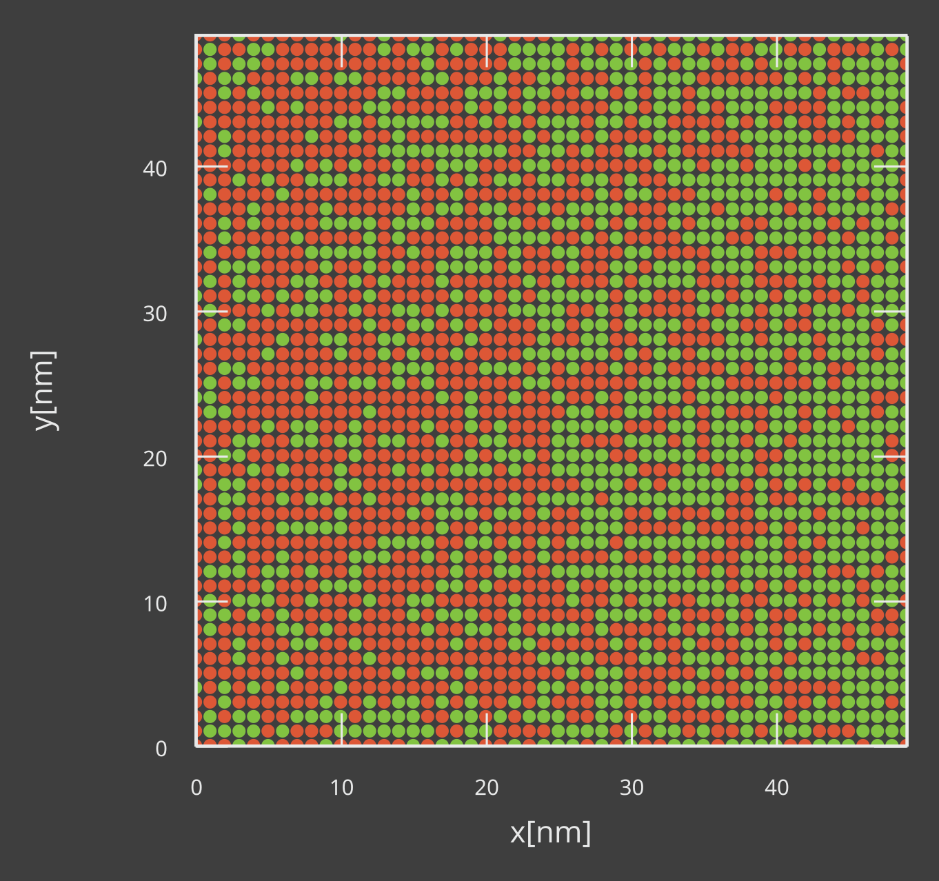
Fig. 62 Layer cross-section for the linear dye gradient

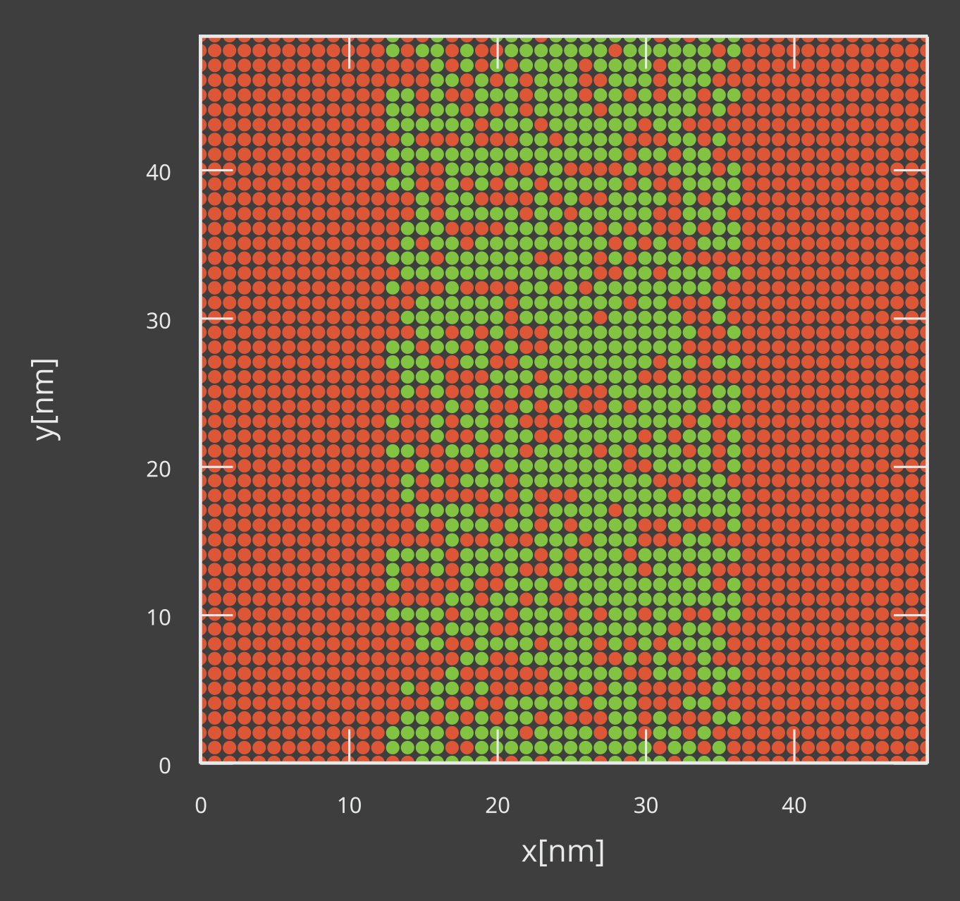
Fig. 63 Layer cross-section for the trapezoidal dye gradient

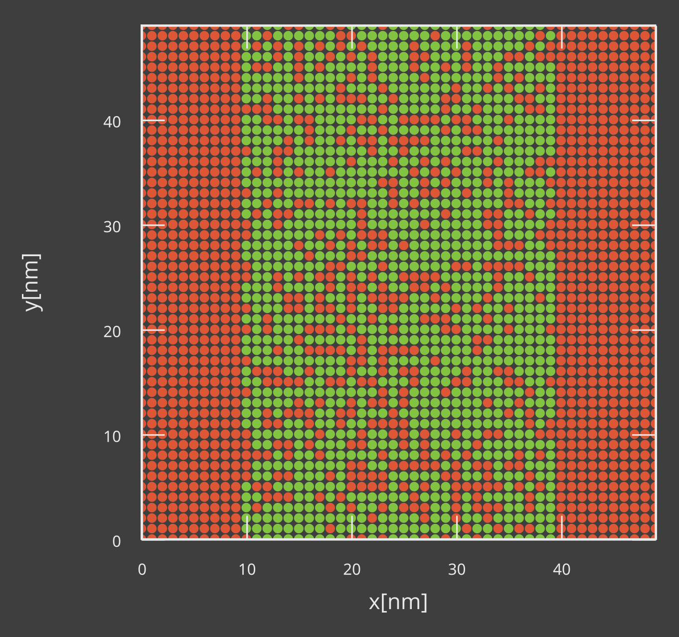
Fig. 64 Layer cross-section for the exponential dye gradient

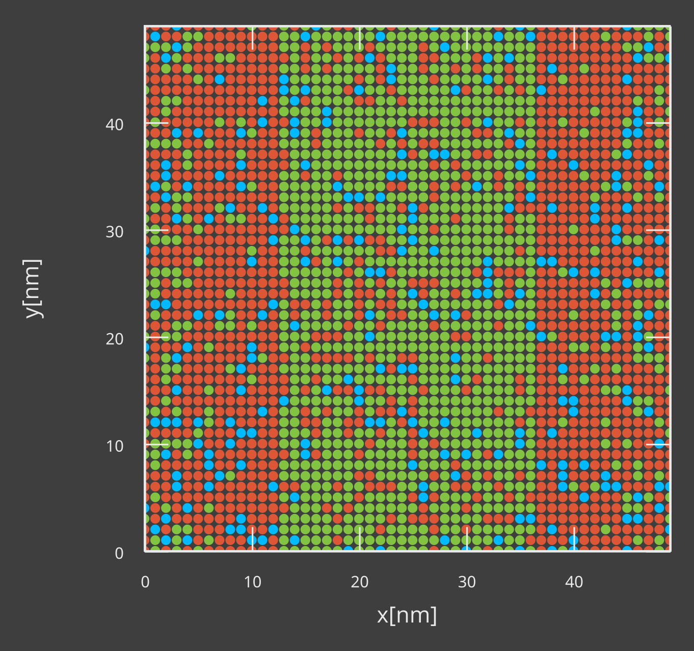
Fig. 65 Layer cross-section for the dual-dye system

Note

The default simulation settings will run 5 trajectories for each job. Each of these will have generated a unique morphology. Note that while the exact distribution of the molecules in the layer is different, the one-dimensional gradient profile (Trajectory → Morphology → Volume Fractions) always matches the prescribed composition.

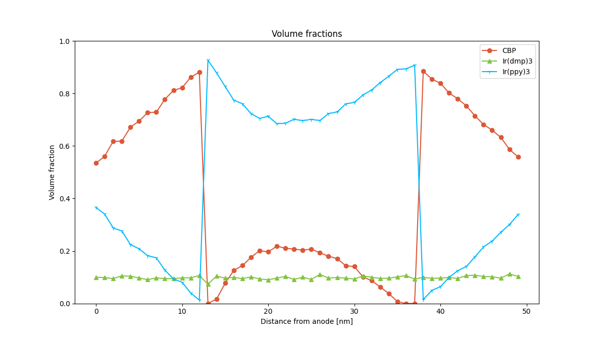
Fig. 66 Volume fractions of the materials in the dual-dye system

Layer Contacts

In order to model the microscopic roughness of layer interfaces, a composite layer can be added to the stack in order to describe the nanoscale spatial mixing of the layer components. For this example, we will look at the interface between a TAPC transport layer and an emissive layer containing a CBP/Ir(ppy)3 host/guest mixture.

We go back to BBinput and navigate to the Composition page. To start, we will define our TAPC/CBP interface. Use the button to add a composition. We use a Basic composition here. (We do not need to enable the advanced generators.)

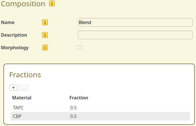
Fig. 67 Material composition for the TAPC/CBP layer interface

Use the button to add 2 materials to the Fractions table. The first material will be set to TAPC, the second material will be CBP. We use a fraction of 0.5 for both materials and use the Save composition button to add the composition to the project.

We will also create our host-guest blend. Use the button to add a composition. We will again use a Basic composition. Use the button to add 2 materials to the Fractions table. The first material will be set to CBP, the second material will be Ir(ppy)3. We use a fraction of 0.9 for CBP and a fraction of 0.1 for Ir(ppy)3. We use the Save composition button to add the composition to the project.

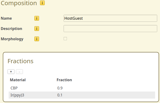
Fig. 68 Material composition for the CBP/Ir(ppy)3 host-guest system

Having created our compositions, we navigate to the Stack page. We will create a new stack containing 3 layers:

• A 20 nm TAPC layer

• A 1 nm layer containing the TAPC/CBP mixture

• A 20 nm layer containing the CBP/Ir(ppy)3 host-guest system

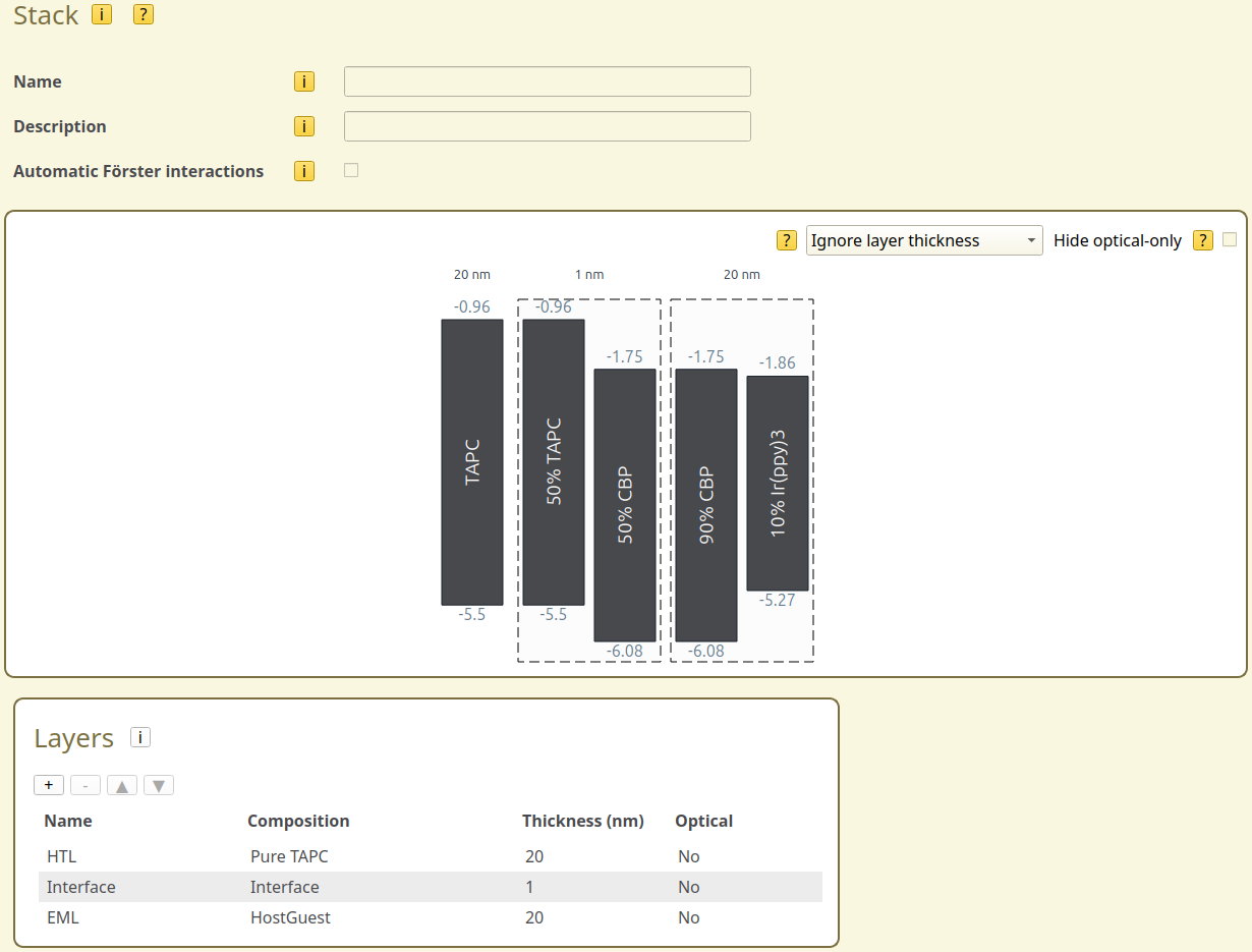
Fig. 69 Setup of the layer contacts in the stack editor

We can use File → Save As → Interface.bee and File → Run to start the simulation.

As seen in BBresults, the resulting morphology localizes the disorder in the interfacial layer.

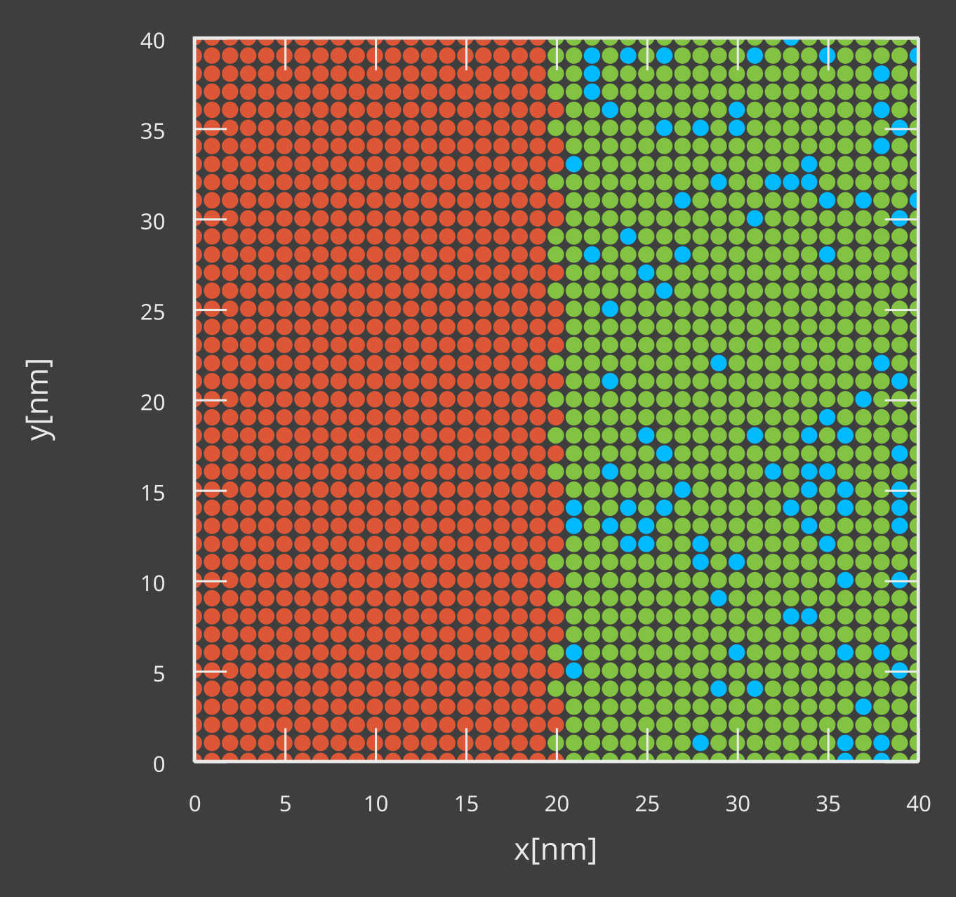
Fig. 70 Layer cross-section for a stack with inter-layer interfacial disorder

The thickness of the TAPC/CBP interface layer can be varied to investigate the effect of the surface roughness on the device.

3D Morphology Generators

In addition to the layer gradients discussed in this tutorial, several specialized generators are also included in the Advanced morphologies.

• The Polymer generator creates polymer networks for PLED devices

• The Quantum Dot generator creates quantum dot lattices for QLED or QNED devices

• The Nanoparticle generator creates nanoparticle or nanocrystallite lattices for HyLED devices

• The Aggregate generator includes self-aggregation of materials that were created by the other generators

These generators create 3D material distributions. (Compared to the 1D profiles obtained by the gradients.) They are designed to replicate the material distributions encountered in specific device types. The application of these generators can be found in the corresponding tutorials.