Bulk Mobility

Periodic boundary conditions can be enabled in order to study the behavior of the bulk material under an active current. In this tutorial, we will determine the electron mobility in TAPC.

Note

A pre-made project file is available for this tutorial.

Create the Material

We will create a new project with BBinput, which can be opened through the SCM → BBinput menu. A new Bumblebee project always requires us to start by defining the materials that will be used in the stack.

Navigate to the Materials page in BBinput and click on the button above the empty material list. Choose the Transport template to set up a material without excitation processes.

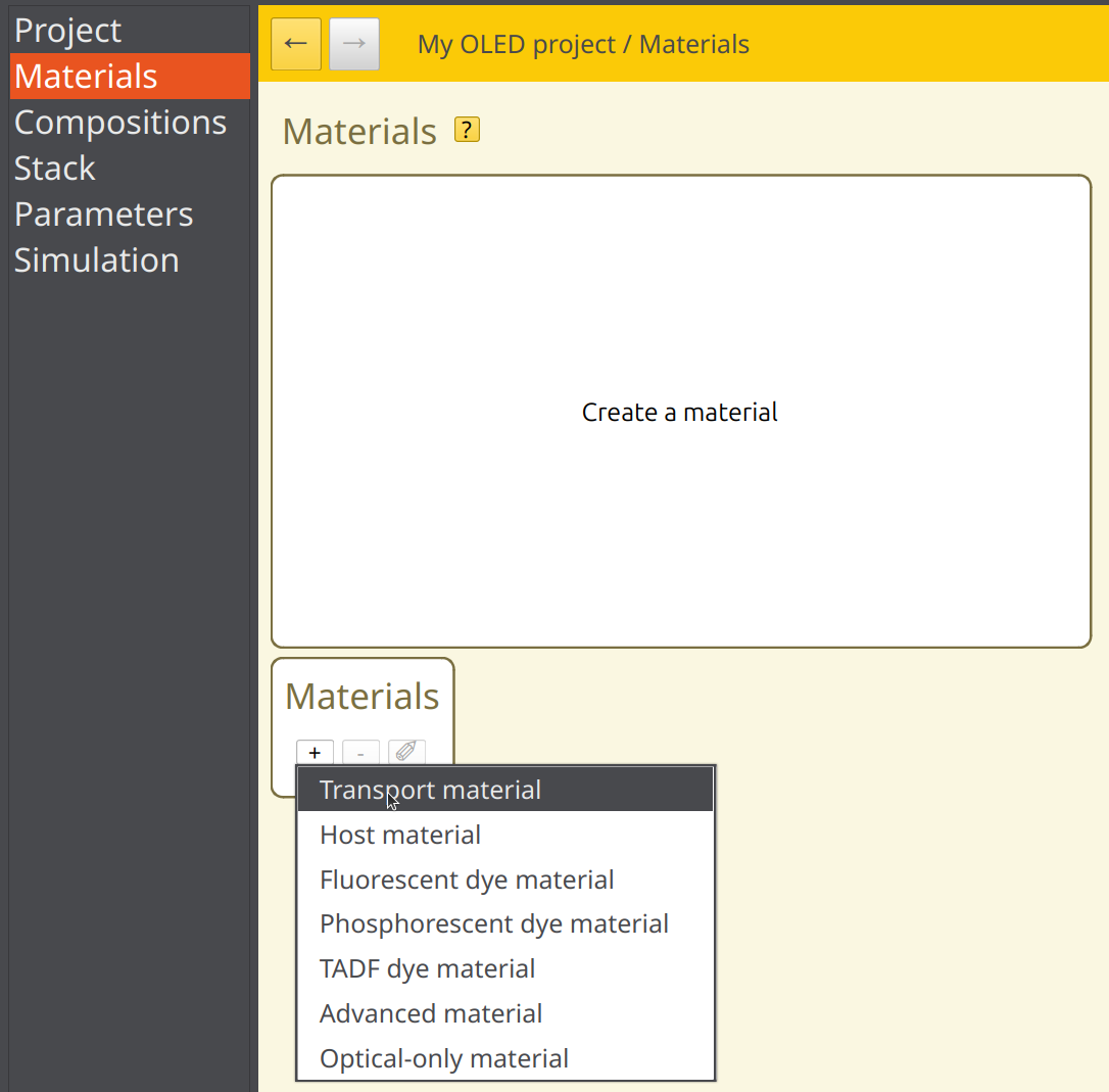
Fig. 6 Create a new material by loading a template

This directs you to the material editor. A Jablonski diagram is shown at the top of the page. The material parameters themselves have been organized in several tabs. You can provide a name for the material on the Main tab.

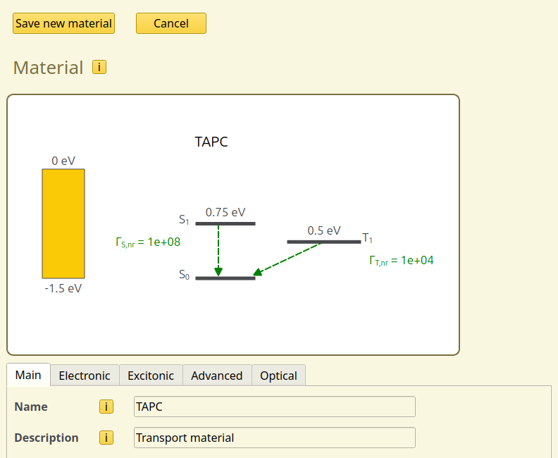
Fig. 7 Material editor after loading the Transport template

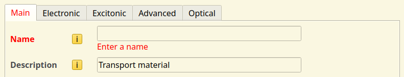
Tip

Tabs containing errors will be highlighted in red.

The Electronic tab specifies the parameters for the polarons (electrons and holes). For this tutorial, we will use a HOMO level of -5.5 eV and a LUMO level of -0.96 eV.

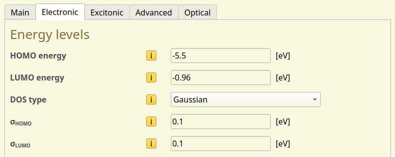
Fig. 8 Polaron settings page for TAPC

The DOS type is used to introduce variations in the energy levels between gridpoints. Due to the amorphous nature of typical OLED materials, the molecular environment differs throughout the layers. These environmental differences affect the inter-molecular interactions, resulting in a distribution of energy levels.

Here, a Gaussian distribution will be used to model this effect. We keep the standard deviations for both HOMO and LUMO levels at 0.1 eV, as this is typical for transport materials.

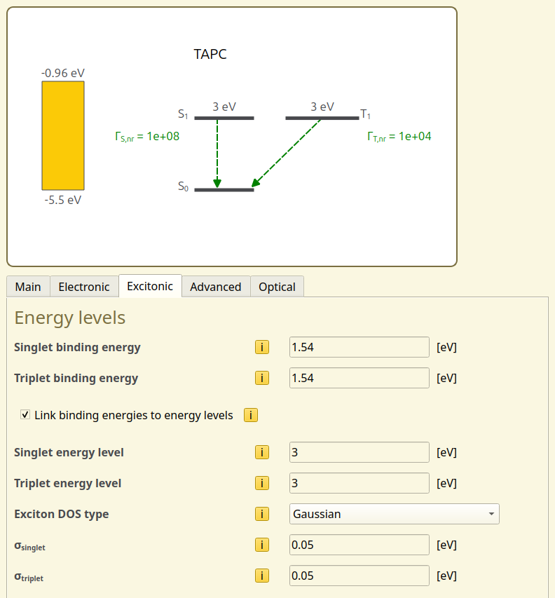
Fig. 9 Exciton settings page for TAPC

The Excitonic tab specifies parameters for the excitons (singlets, triplets) and the excitation processes. As we will not be modeling excitons in this tutorial yet, simply set the singlet and triplet energy levels to 3 eV. The binding energies are updated automatically. We then use the Save new material button at the top of the page to add TAPC to the project.

Whenever a new material is created, a pure composition is also added to the Compositions page. Compositions are used to create blends of multiple materials for use in the OLED layers. Pure compositions only contain a single material, and allow you to directly use the new materials when designing the OLED stack.

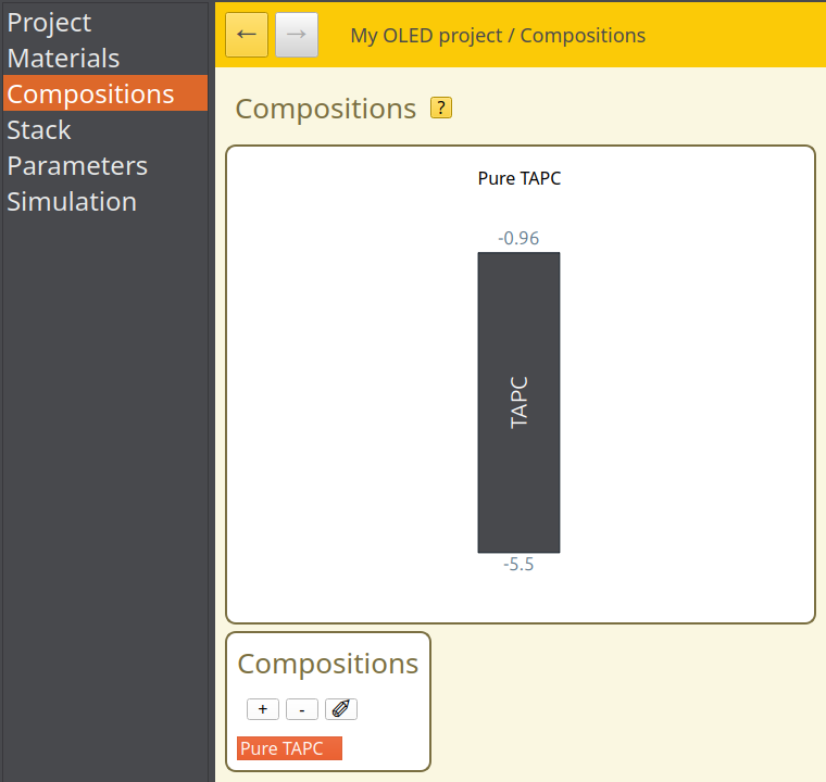
Fig. 10 Pure compositions are automatically created for new materials

Create a Stack

After defining the materials and compositions, we can now create an OLED stack by defining the layers. Here, we will be using only a single layer in order to model the bulk material behavior.

Navigate to the Stack page in the GUI. This will open the stack editor, which allows us to define the layers. As before, provide a name for the stack. Then click on the button in the Layers table. A new layer will be added to the stack diagram. The Layers properties can be edited by selecting a parameter in the table. The TAPC material has been set automatically, so we only need to update the thickness. For this tutorial, we will use a bulk system of 50 nm. Click the Save stack button to save your changes.

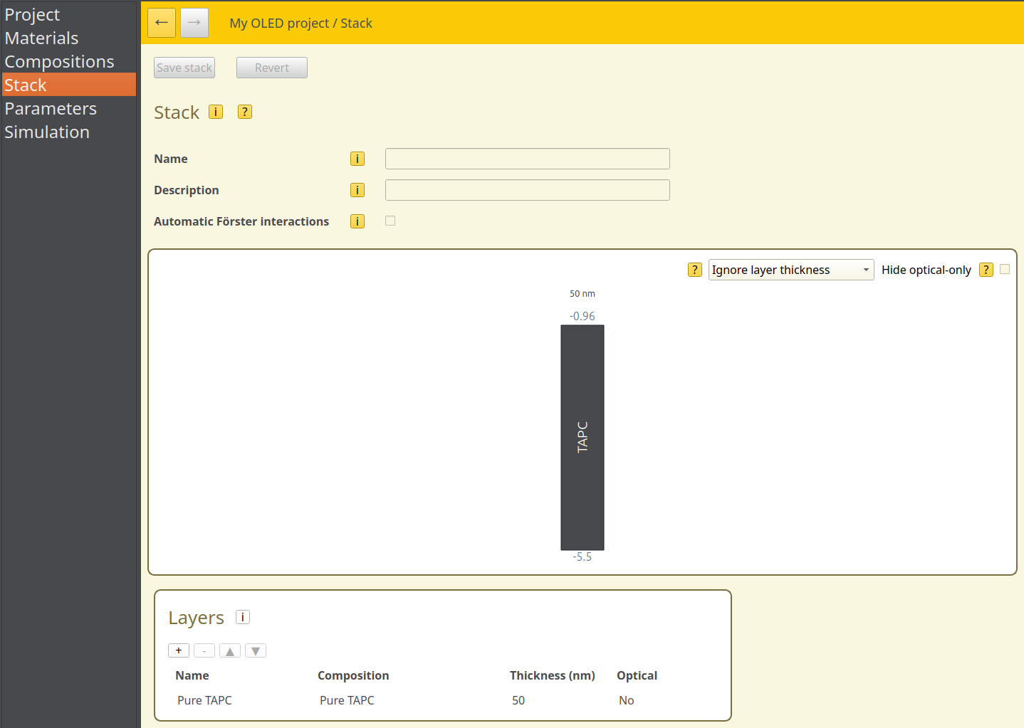
Fig. 11 Stack editor layout for the single TAPC layer. Hovering over the stack diagram shows the material properties

The remaining sections of the stack editor relate to the excitonic processes, so we can leave these alone for now.

Create a Parameter Set

Having created the OLED stack, we will now configure the simulation settings. Navigate to the Parameters page and click on the Load preset button. This will open a selection of simulation templates. As we are modeling a bulk material, select the Bulk Simulation template. This will automatically configure some of the parameters required for modeling bulk systems.

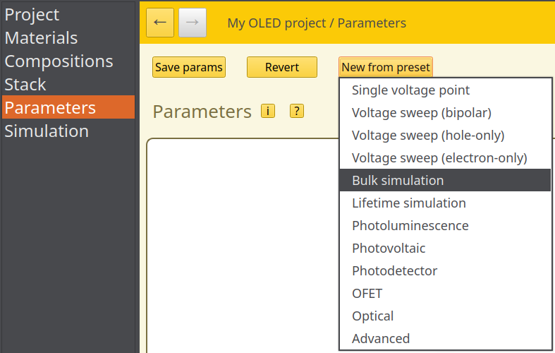
Fig. 12 Parameter set template selection

Device Parameters

In the Main tab, provide a name for this parameter set.

In the Physical Parameters section of the Main tab, we can set the device voltage. We will use 1 V for this simulation. Keep the temperature at 300 K. The dielectric constant is used to set the effective permittivity of the device (i.e. for all the layers in series). For now, we will use a default value of 3.

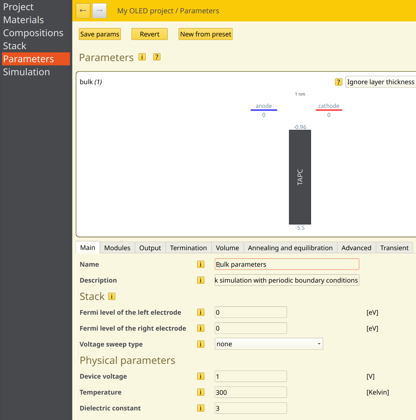
Fig. 13 Overview of the device parameters

Simulation Volume

The device geometry is described in the Volume tab. Periodic boundary conditions should have been enabled by default when using the Bulk simulation template. This will enable us to model charge transport in a semi-infinite bulk medium.

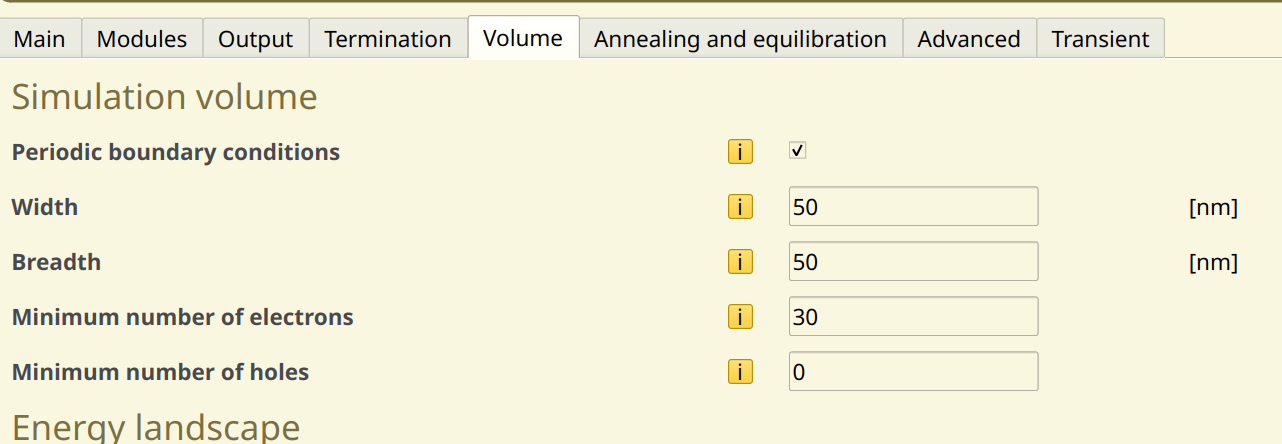
Fig. 14 Simulation volume settings

The number of sites determines the simulation grid and sets the size of the modeled surface area of the cell. We will use the default of 50 nm in both directions.

Because we are modeling the bulk of the device using periodic boundary conditions, this means that the electrode contacts are not included in the simulation grid. A fixed number of polarons will therefore be used to investigate charge transport. We will use a single polaron type for this tutorial by setting the number of electrons to 30 and the number of holes to 0.

Simulation Duration

The settings in the Termination tab specify how long the simulation will run.

As Bumblebee determines the device performance through stochastic sampling, it is important that a sufficient number of steps is allowed in order to provide accurate statistics. This can be achieved in 2 ways:

• Increase the number of steps in the simulation

• Perform multiple simulations in parallel and collect the results (this can be enabled during the job submission step)

For this tutorial, we will set the Number of simulation steps to 30,000,000. This is the maximum number of steps that the simulation will go through. Additional convergence criteria can be specified to allow early termination. These can be left off for now.

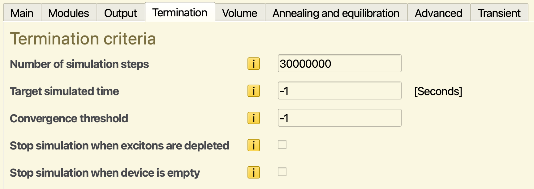
Fig. 15 Termination criteria

Tip

As the required number of steps is not known beforehand, it is typical to use a high step limit as a default. The simulation can be monitored with BBresults, and the simulation can be stopped manually once the properties of interest have converged.

Output Settings

The Output tab allows specifying the frequency with which simulation results are reported. This frequency is set separately for 2 types of files:

• The report interval determines how often the simulation summary and log files are updated

• The output interval determines updates to the remaining output files

Writing output to a large number of files can slow down the simulation significantly. For this reason, the output interval is often taken to be larger than the report interval. Individual output files can also be enabled or disabled manually in the Output tab to reduce the cost of writing files.

For this tutorial, we will set a report interval of 5,000 steps and an output interval of 100,000 steps.

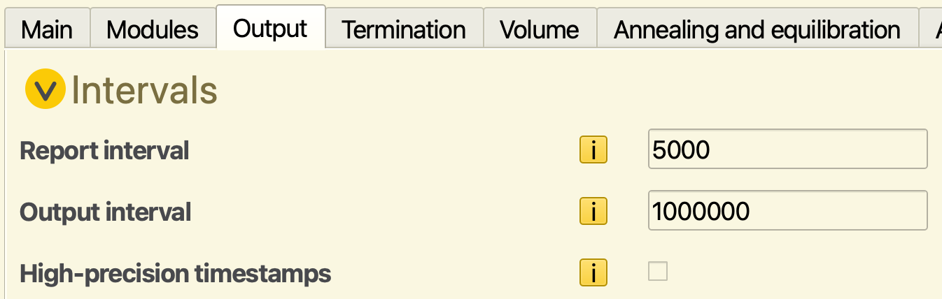
Fig. 16 Output settings

Finally, press the Save parameters button to apply the changes to the project.

Starting the Simulation

The Simulation tab allows submitting simulation jobs using the previously specified parameter set.

Multiple trajectories can be run in parallel. This allows you to split up the sample generation between multiple independent simulations. Each trajectory has a different initial state and a different distribution of energy levels, thereby effectively increasing the size of the simulated surface area. Bumblebee will automatically collect sample data from each simulation and include this data in the device statistics.

We will select 2 trajectories in order to illustrate this process (without using too many resources). To obtain better statistics, you can increase the number of trajectories here, or the simulation time in the parameter set. Note however, that this will also increase the computational cost of the simulation.

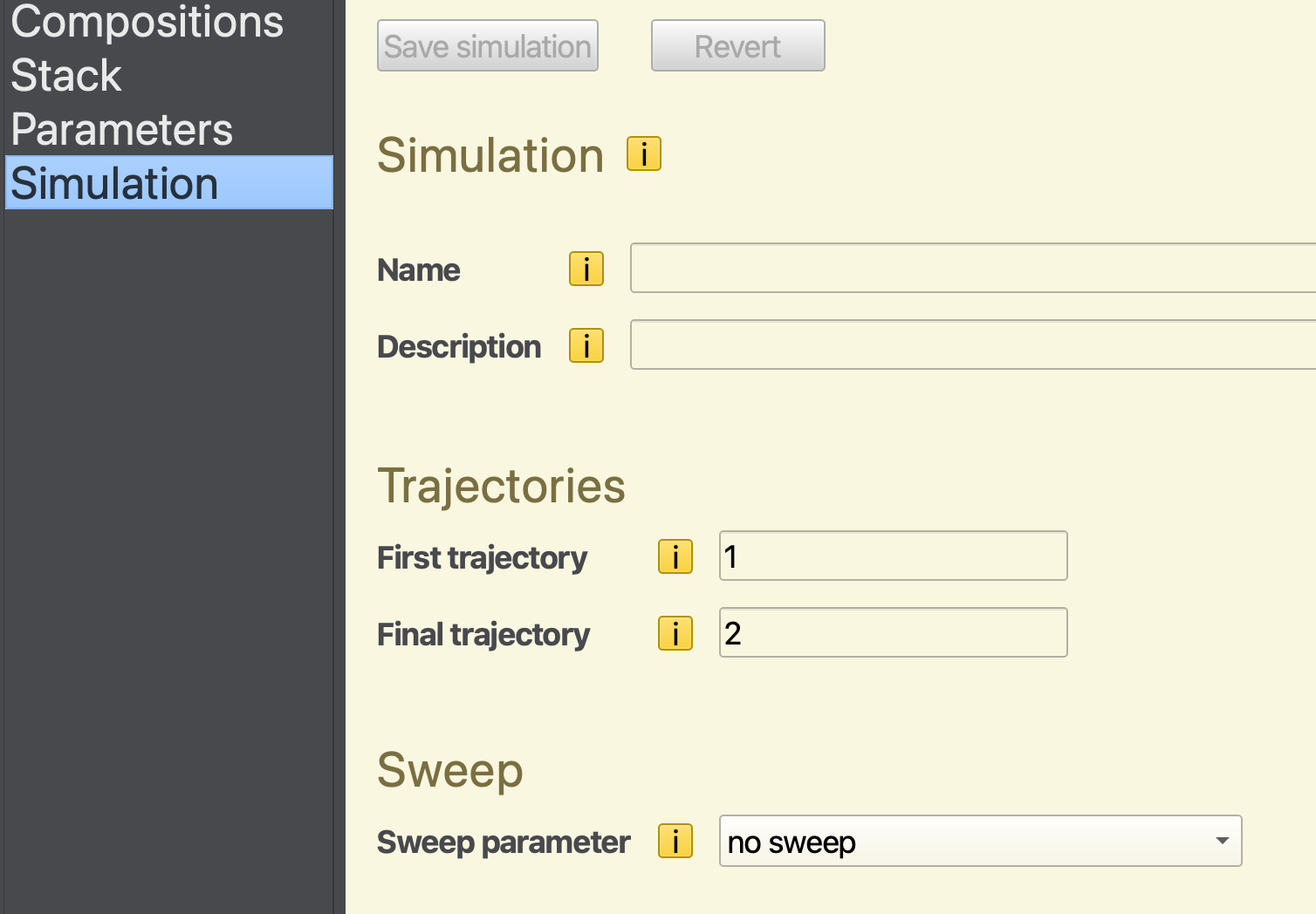
Fig. 17 Trajectory and parameter sweep configuration

The sweep parameters will not be used for this tutorial.

We now save our project to a (.bee) file by selecting File → Save from the main menu. You can start the simulation by selecting File → Run. If you want to switch to a remote queue, you can also start the simulation through AMSjobs instead.

Monitoring the Simulation

After starting the simulation, we can use BBresults to monitor the output. From BBinput, select SCM → BBresults to automatically open the associated results folder.

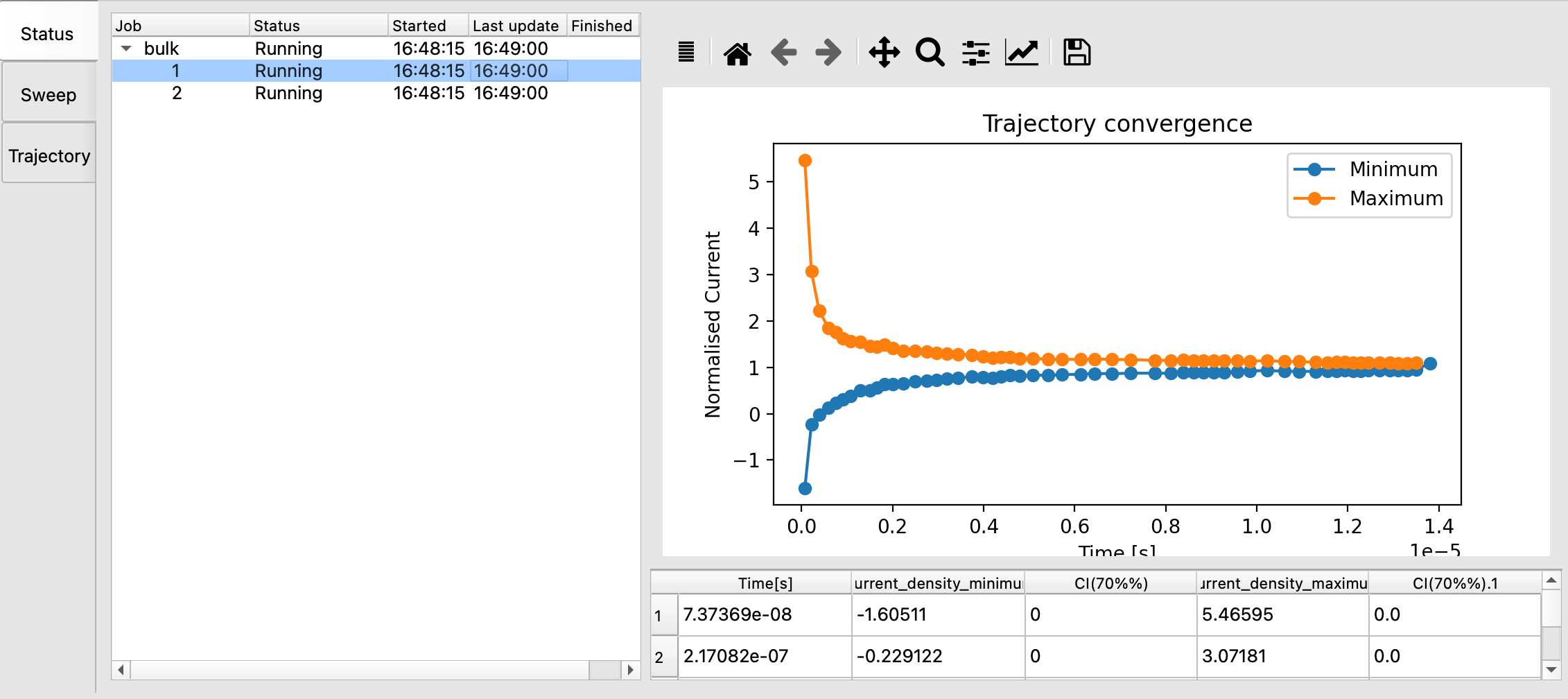
Fig. 18 Progress of a running Bumblebee job in BBresults

The main page of BBresults shows an overview of the active trajectories (and parameter sweeps, if enabled). The convergence of the simulation is measured by looking at the changes in the device current. Bumblebee compares the measured current at every point along the length of the device. A trajectory has reached steady-state once the two lines meet, at which point the current density is constant throughout the stack.

By selecting one of the trajectories in the list, we can view the convergence of the current for this particular simulation. The graph will automatically update as the simulation advances.

A table containing the raw data is also provided for each graph in BBresults. This allows retrieval of specific numerical data and allows exporting of the results to external visualization or analysis programs.

Simulation Results

The Device, Sweep and Trajectory panels in BBresults provide visualization and analysis of the simulation output. For bulk simulations, we are interested in the charge carrier mobility. This can be found in the Device → Effective Mobility tab:

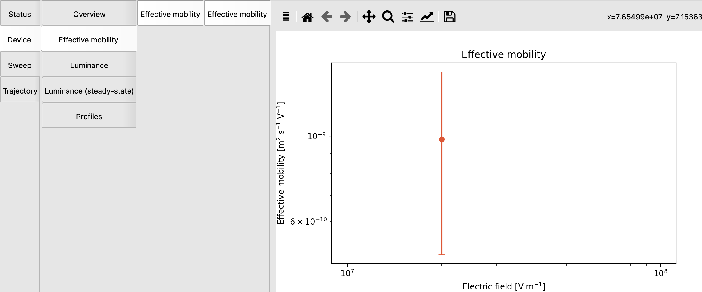
Fig. 19 The effective mobility of electrons in the TAPC material after 4 μs

The effective mobility graph contains a single datapoint, corresponding to our simulation at 1.0 V. An error bar is provided to show the statistical uncertainty in the predicted mobility. These errors are obtained by analyzing the variations in mobilities predicted by the 2 trajectories.

As the simulation progresses, we find that the error is reduced with an increasing sample count, as the simulation progresses towards the steady state.

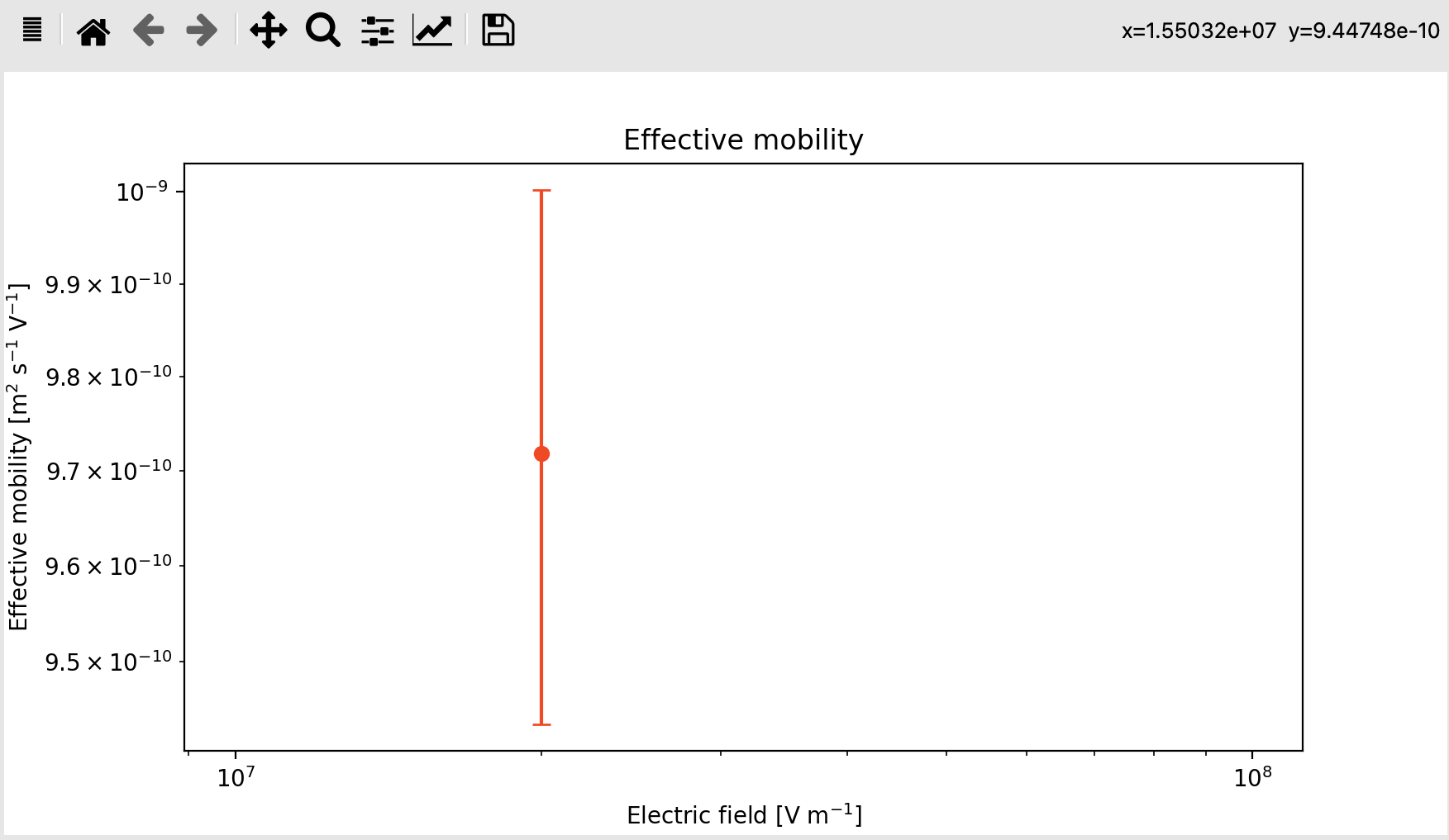
Fig. 20 The effective mobility after 45 μs

We can see that the estimated value for the electron mobility falls in line with experimentally reported data.

Note

We can vary the voltage in order to see how the mobility changes as a function of the applied potential. Comparison with experimentally measured zero-field mobilities can be done by extrapolating the predicted mobility towards zero voltage.

The number of charges can also be changed to investigate how the charge density affects the mobility in the device.

Extending the Simulation

We have seen that an increased number of samples helps improve the accuracy of the calculated properties. In order to reach the required number of samples, there are 2 options:

• Keep the simulation running for a large number of steps

• Run multiple trajectories in parallel

Sometimes, a simulation may take a relatively long time to converge. This also means that a large number of simulation steps could be required to reduce the error bars. By using multiple trajectories, we can reduce the total simulation time by running multiple simulation in parallel.

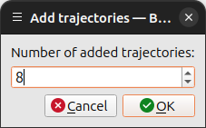
BBresults allows you to add additional trajectories, even if the simulation has already started. Select Simulation → Add trajectories and set the appropriate number. We will request 8 new trajectories.

The Status page in BBresults will be updated to include the new trajectories. The graphs shown in BBresults will also be updated automatically to include the new data once these simulations start running.

The most notable improvement obtained by running additional trajectories can be seen in the transient data, where averaging over multiple trajectories helps in denoising the profiles. We can observe this by comparing the transient current profiles, found in the Sweep → Overview → Current tab.

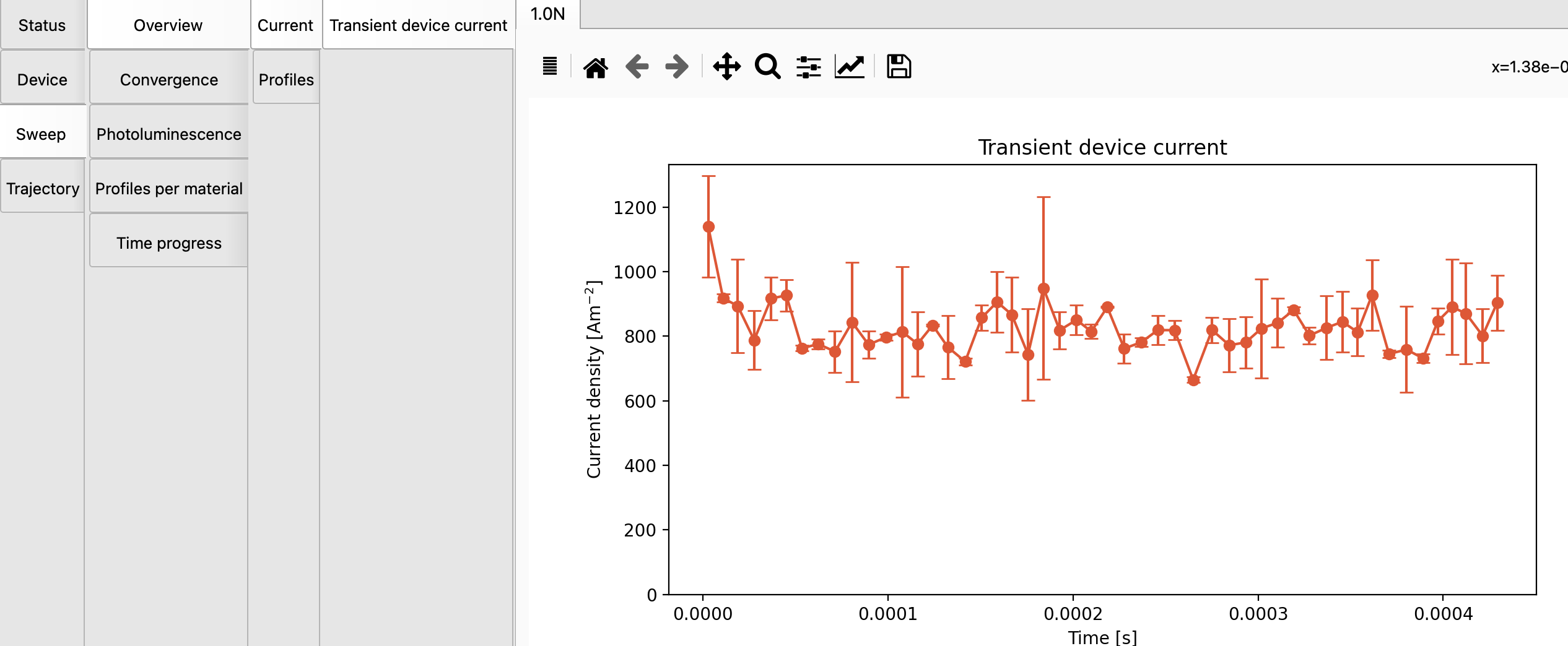
Fig. 21 Transient device current averaged over 2 trajectories

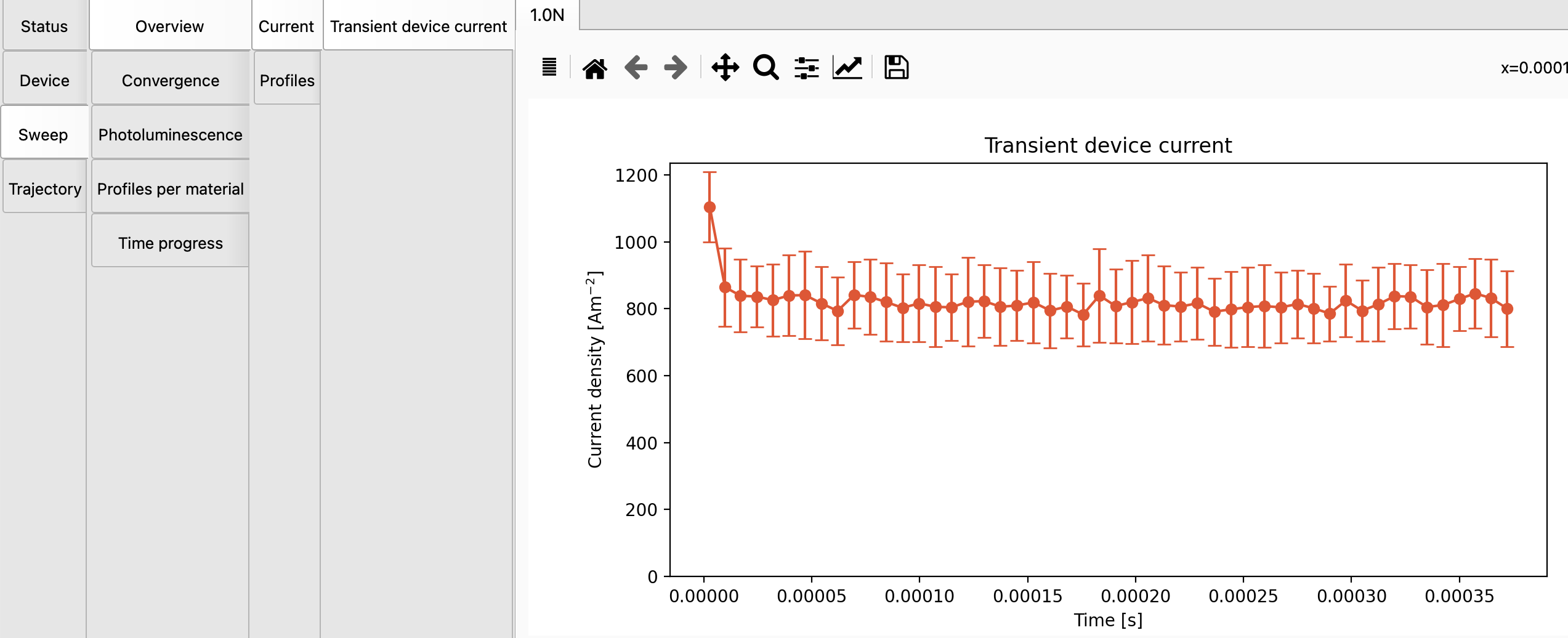
Fig. 22 Transient device current averaged over 10 trajectories

Note

Each trajectory generates a new sampling of the amorphous disorder. The morphology, DOS and orientation factors will be unique for each trajectory.

An increased number of trajectories can also be interpreted as sampling over a larger OLED surface area (or a larger volume, in case of bulk simulations).

For strongly disordered systems, or materials containing low trap concentrations, this increased volume sampling may be required to properly capture the inhomogeneity in layer properties.

Stopping the Simulation

In this tutorial, we have requested a simulation that runs for a large number of steps. When monitoring the output we can look at:

• The trajectory convergence on the Status page

• The error estimate (error bars) of the mobility (our target property)

Once the current has reached steady-state, and the mobility prediction is accurate enough, we can request an early stop for the ongoing simulation.

In BBresults, you can select trajectories on the main Status page. Right-click and Request stop to trigger an early stop for these simulations. (The other trajectories will be unaffected and continue running.) You can also access this option from the Simulation → Request stop menu.

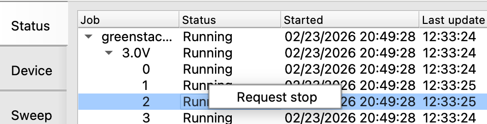
Fig. 23 Request trajectory termination from the Job Status panel in BBresults

When an early stop is requested, Bumblebee will wait until the ongoing steps have finished. Residual data is collected and written to file before the simulation is fully stopped. This prevents any data loss in case a trajectory is terminated through BBresults.

Once you are done with this tutorial, feel free to use the Simulation → Request stop all option to wrap up the simulation.