Polymeric OLED¶

For polymeric OLED materials, the charge transport along the polymer backbone can differ from the transport between adjacent chains. Polymeric morphologies can be created to account for this behavior during Bumblebee simulations.

Create Materials¶

We will create a new project with BBinput, which can be opened through the SCM → BBinput menu. On the Materials page, we start by defining the layer materials.

Polymer¶

In this tutorial, we will consider a SY-PPV PLED. We start by generating a new material for the polymer. Use the AddButton button to open the material editor for a new material. We use the Fluorescent Dye template here.

We set a HOMO level of -5.4 eV and a LUMO level of -2.8 eV. For the polymer, we will disable the energy level broadening by setting DOS type to Delta. For the excitons, we use a singlet binding energy of 1.3 eV and a triplet binding energy of 1.6 eV. A delta function is again used as Exciton DOS type to disable energy level broadening.

An enhanced Singlet fraction for exciton generation of 0.4 will be used. For singlets, the radiative decay rate is set at \(10^{8}\,\textrm{s}^{-1}\) and the non-radiative decay rate is set at \(5\cdot{}10^{7}\,\textrm{s}^{-1}\). We leave both triplet decay rates at the default values.

To describe the preferential carrier hopping along the conjugate backbone, anisotropic hopping rates can be specified in the Advanced tab of the materials editor.

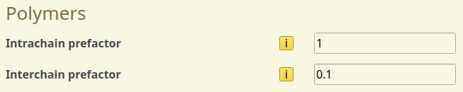
../_images/advanced_tab_75ba7782.png — Fig. 71 Charge transport anisotropy settings for polymeric materials¶

We chose here to set an interchain prefactor of 0.1 to suppress charge hopping between the chains.

Vacuum Level¶

Due to the imperfect stacking of polymer chains in the emission layer, voids will be present between the chains. To account for this, we create a vacuum material to represent these voids using the Advanced material template.

We set a HOMO level of 25 eV and a LUMO level of 50 eV. Energy level broadening is disabled using DOS type = Delta. This choice of energy levels creates a large barrier for transfer towards the vacuum, preventing this material from participating in electron transport.

Because the vacuum should not carry any excitons either, the singlet and triplet binding energies can be set to 0. Energy level broadening is disabled by Exciton DOS type = Delta.

To inhibit transport, the hole mobility, electron mobility and both Dexter prefactors are set to 0 on the Excitonic tab.

Transport Layer¶

PEDOT:PSS will be used as a hole transport layer. We select the Transport template to create a new material.

We set a HOMO level of -5 eV and a LUMO level of -2.3 eV. A Gaussian energy level broadening is enabled by default. For the excitons, we use a singlet binding energy of 0.7 eV and a triplet binding energy of 1.2 eV.

Create a Polymer Network¶

In order to include the morphology of the polymer network, we will create an advanced composition.

Go the Composition page and select the AddButton to create a new layer composition. In the composition editor, select the Morphology option to access the advanced composition generators. We will use these to create a 3D network of polymeric chains.

Select the vacuum as the background material and use the AddButton button in the Morphology table to add a generator. Change the material to SY-PPV in the table and select the Polymer generator option by double-clicking the Linear gradient field. A new editor for the polymer generator will appear below the table.

The polymer generator will attempt to fill the layer using polymeric chains obtained through a self-avoiding walk. A polymer fraction is specified to determine the portion of the grid that will be filled with the polymeric material. The maximum size of the individual chains is set using the chain length parameter. Note that not every polymer will be able to reach the maximum chain length, either due to confinement by neighboring chains or the finite size of the layer.

The behavior of the self-avoiding walker is set using an anisotropic growth vector, which describes the relative probability that chains grow in any given direction. The rigidity parameter restricts the polymer chain from folding back onto itself within a set number of backbone units.

For SY-PPV, we will use a polymer fraction of 0.8, a chain length of 25 and a backbone Rigidity of 4. The chain growth probability towards the electrodes will be doubled using Growth rate (x) = 2 in order to generate a directed conductor.

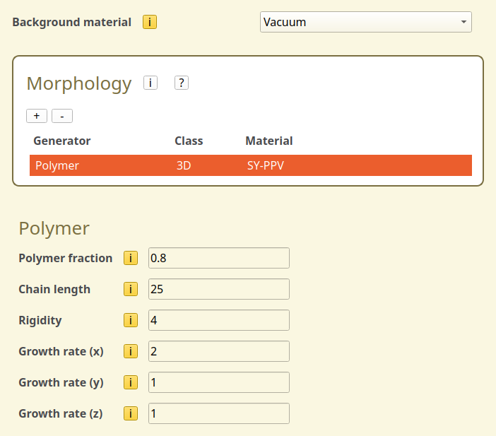
../_images/polymer_generator_efcd3a0f.png — Fig. 72 Polymer generation settings¶

Create a Stack¶

We will create a stack containing 2 layers. The electron transfer is assumed to proceed through a metallic contact.

Add a 20 nm layer of PEDOT:PSS
Add a 60 nm layer of the polymer composition

We use the Add default interactions option in the Förster interactions table to automatically configure the excitonic mechanisms. Use the DeleteButton button to remove any processes that involve the vacuum.

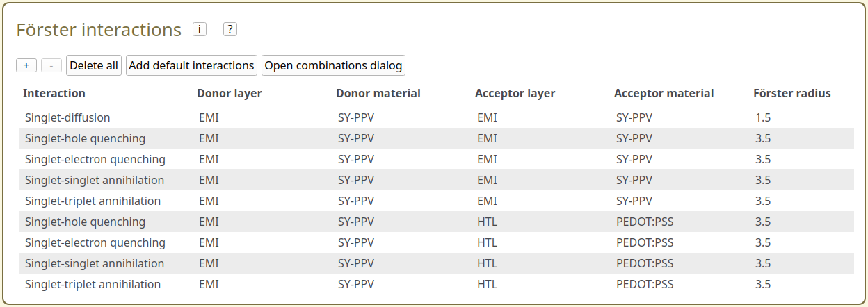
../_images/default_foerster_7193abd6.png — Fig. 73 Förster interactions overview in the stack editor¶

Create a Parameter Set¶

On the Parameters page, we use the Load preset button to select the Single Voltage Point template.

The device voltage will be set to 5 V. Because the polymer layer contains voids, we have to manually set the electrode energy levels. We use an energy of -4.8 eV for the anode and -3.0 for the cathode.

Finally, we switch to the Modules tab and tick the Excitonics checkbox to enable exciton modeling.

Starting the Simulation¶

For this tutorial, we will set up a new simulation for a single voltage point.

On the Simulation page, we select 5 trajectory instances to improve the sampling of the polymer network. The Sweep is set to None as we only want to run the simulation for a single set of parameters.

We can now use File → Save and File → Run to start the simulation.

Simulation Output¶

The morphology of the polymer layer can be viewed in the Trajectory → Morphology → Device → Cross-section tab of BBresults.

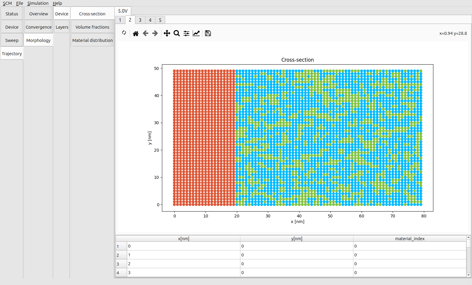
../_images/morphology_737948eb.png — Fig. 74 Layer cross-section for the PEDOT:PSS/SY-PPV stack (Red = PEDOT:PSS, Blue = SY-PPV, Green = Void Fraction)¶

The labeled tabs above the graph can be used to change between the morphologies that were generated for the different trajectories. Each graph shows a cross-section of the device.

The precise morphology differs per trajectory, which allows us to account for the variations in the network structure. (Effectively, we have increased the simulated surface area of our PLED.) From the shape of the voids in the cross-sectional view, we can see the preferential alignment of the polymer chains along the X-axis, in line with the distribution specified for our network generator. Along with the preferential intrachain charge transport along the polymer backbone, this shortens the effective path length between the electrodes, which is in turn reflected in the Trajectory → Convergence → Overview reports.