Example: TD-CDFT for bulk silicon (OldResponse)
The time-dependent current DFT functionality, as implemented by Kootstra, Berger, and Romaniello, enables you to calculate frequency-dependent dielectric functions for 1-dimensional and 3-dimensional periodic systems. In the present example, a standard geometry for bulk Silicon is given. The important part in this example is of course the OLDRESPONSE key block. It specifies that 7 frequencies shall be computed, with an even spacing between 0.0 eV and 6.8 eV. In this example scalar ZORA relativistic effects are switched on with the isz line in the OLDRESPONSE key block.
$ADFBIN/band << eor
DefaultsConvention pre2014

TITLE Silicon

ACCURACY 5
KSPACE 2

DEPENDENCY BASIS 1e-10

UNITS
   LENGTH ANGSTROM
END

OLDRESPONSE
   nfreq   7
   strtfr  0.0
   endfr   6.80285
   isz     1
END

DEFINE
   AAA=5.43
   HA=AAA/2
END

LATTICE
   0   HA  HA
   HA  0   HA
   HA  HA  0
END

ATOMS
   Si  0.0   0.0   0.0
   Si  HA/2  HA/2  HA/2
END

END INPUT
eor
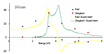
For Silicon the real and imaginary parts of the dielectric function:
are calculated.
In the output file, the results will look something like the fragment below. The output specifies for which frequency the dielectric function is determined, and then proceeds to print the values for the 3x3 tensors.
The real and imaginary parts are printed separately. At this frequency, the imaginary part is still zero. Because of the high symmetry of the system, the real part is a constant times the unit matrix except for numerical noise.
 Frequency    0.833333E-01 au    2.26756     eV
 Start the SCF procedure
* Real
 Chi_jj   X     -12.8363       0.142802E-18   0.547977E-17
 Chi_jj   Y     0.202883E-17   -12.8363       0.121052E-17
 Chi_jj   Z     0.124042E-16   0.215311E-17   -12.8363
* Imag
 Chi_jj   X     0.000000E+00   0.000000E+00   0.000000E+00
 Chi_jj   Y     0.000000E+00   0.000000E+00   0.000000E+00
 Chi_jj   Z     0.000000E+00   0.000000E+00   0.000000E+00
*
After each frequency has been treated, the results are summarized for each main diagonal component separately in a table. The frequency/energy is again printed in two different units, the Dielectric Function is printed in a.u. The values for Chi, which are trivially related to those printed here, are summarized in a separate table.
=================================================================
==         Frequency         ===       Dielectric Function     ==
==     a.u.   ==      e.V.   ===        Re    ==        Im     ==
============XX-dir===============================================
    0.416667E-01     1.13378         16.1119        0.000000E+00
    0.833333E-01     2.26756         23.7904        0.000000E+00
    0.125000         3.40134         15.8529         35.8574
    0.166667         4.53512        -3.49949         20.2221
    0.208333         5.66890        -6.60897         12.3661
    0.250000         6.80268        -6.42943         6.87957
============YY-dir===============================================
    0.416667E-01     1.13378         16.1119        0.000000E+00
    0.833333E-01     2.26756         23.7904        0.000000E+00
    0.125000         3.40134         15.8529         35.8574
    0.166667         4.53512        -3.49949         20.2221
    0.208333         5.66890        -6.60897         12.3661
    0.250000         6.80268        -6.42943         6.87957
============ZZ-dir===============================================
    0.416667E-01     1.13378         16.1119        0.000000E+00
    0.833333E-01     2.26756         23.7904        0.000000E+00
    0.125000         3.40134         15.8529         35.8574
    0.166667         4.53512        -3.49949         20.2221
    0.208333         5.66890        -6.60897         12.3661
    0.250000         6.80268        -6.42943         6.87957
Results of the test calculation (red/blue) are plotted in next Figure together with experimental data (yellow/green). The results for the seven specified frequencies are given. It should be obvious that more frequencies are needed (resulting in longer run times) to obtain a smooth curve in which peaks cannot be missed because of too coarse interpolation.