Python scripting for COSMO-RS with PLAMS
General Information
Attention
Windows and Mac users may find it helpful to first read the Getting Started guides for scripting: scripting with Windows | scripting with MacOS
Python and the PLAMS library can be used for scripting with COSMO-RS. Due to the speed of COSMO-RS calculations, these jobs can be run interactively from the python interpreter. Larger numbers of jobs or high-throughput calculations can also easily be automated with python scripting. All results are returned as a python object, meaning the properties calculated with COSMO-RS can immediately be post-processed or used directly in other python functions.
Note
COSMO-RS calculations require a .coskf or .compkf file for every compound in the system. .coskf and .compkf files only need to be calculated once and then are stored in a database and can be used for any future calculation containing the corresponding compound. Generating these files requires calculating the COSMO surface with ADF (a relatively more expensive DFT calculation). Setting up these calculations is not directly supported with this version of PLAMS but can be done using scripting with adfprep.
Executing the code from the command line
It is recommended to use the version of python that is shipped with AMS. This version ensures that all the necessary libraries (e.g., PLAMS) are properly imported and are mutually compatible. The best way to do this is to run AMS’s startpython program. That can be executed from the command line as follows:
$AMSBIN/startpython <your_program.py>
where <your_program.py> should of course be replaced by the name of your program.
Specifying a problem type
To run COSMO-RS, the user must first provide a problem type for the calculation. This can be done by first creating a Settings object and then specifying the .input.property._h attribute. For example, to set up an activity coefficient calculation, we do the following:
from scm.plams import *

settings = Settings()
settings.input.property._h = 'ACTIVITYCOEF'
For other problem types, the .input.property._h attribute must be set to other values. The other options for this value are summarized below:
._h value |
Problem type |
|---|---|
| ACTIVITYCOEF | Activity Coefficient |
| BINMIXCOEF | Binary mixture LLE/VLE |
| TERNARYMIX | Ternary mixture LLE/VLE |
| COMPOSITIONLINE | Solvent composition line interpolation |
| SOLUBILITY | Solubility calculation in a mixed solvent |
| PURESOLUBILITY | Solubility calculation in a pure solvent |
| LOGP | Partition coefficient calculation |
| VAPORPRESSURE | Vapor pressure calculation for a mixed solvent |
| PUREVAPORPRESSURE | Vapor pressure calculation for a pure solvent |
| BOILINGPOINT | Boiling point calculation for a mixture |
| PUREBOILINGPOINT | Boiling point calculation for a pure solvent(s) |
| FLASHPOINT | Flashpoint calculation for a mixture |
| SIGMAPROFILE | Sigma profile calculation for a mixture |
| PURESIGMAPROFILE | Sigma profile calculation for a pure component(s) |
| SIGMAPOTENTIAL | Sigma potential calculation for a mixture |
| PURESIGMAPOTENTIAL | Sigma potential calculation for a pure component(s) |
Inputting Compounds
In PLAMS, each compound is also input as a Settings object. Additional information about the compounds required for the calculation (e.g., mole fraction) can be specified as an attribute of the compound’s Settings object. An example for a calculation with two compounds is given below.
# set the number of compounds
num_compounds = 2

compounds = [Settings() for i in range(num_compounds)]
compounds[0]._h = "Water.coskf"
compounds[1]._h = "1-Hexanol.coskf"
Specifying mole fractions, temperatures, and pressures
Mole fractions are attributes of the compound Settings object. There are two types of mole fractions used in COSMO-RS. frac1 is for standard specification of mole fractions in most problem types. frac2 is used when the problem type requires two distinct liquid phases (COMPOSITIONLINE or LOGP). Additionally, the temperature can be specified using the input.temperature attribute of the Settings object. An example of this is shown below:
#set compound mole fractions
compounds[0].frac1 = 0.3
compounds[1].frac1 = 0.7

#set temperature (range)
#to specify a range, use 3 numbers: (1) the lowest temperature,
#(2) the highest temperature, and (3) the steps taken between these temperatures
settings.input.temperature = "298.15"
To specify a temperature range, set the input.temperature object equal to a python str which contains the lower temperature, upper temperature, and number of steps taken between the temperatures. These values should simply be separated by spaces. For example, to specify that a calculation should go over the temperature range 298.15K to 398.15K with 10 temperature steps, do the following:
settings.input.temperature = "298.15 398.15 10"
Pressure works in much the same way. To input the system pressure (in bar), do the following:
settings.input.pressure = "1.5"
Running jobs
To run a job with COSMO-RS, first assign the input.compound attribute to the list of compound Settings objects used previously. Then, simply create the job using CRSJob(settings=<your previously defined Settings object>). Once a job is created, you can run it with the .run() function. An example of this is given below:
# specify the compounds as the compounds to be used in the calculation
settings.input.compound = compounds
# create a job that can be run by COSMO-RS
my_job = CRSJob(settings=settings)
# run the job
init()
out = my_job.run()
finish()
Reading the results of a job
Once a job has finished running, we can access the results directly in python. First, we can check to see which properties are available. We can do this using the get_prop_names() function on the output. For example, adding the line:
# check for the available properties
print( "Available properties:", out.get_prop_names() )
gives us the available properties as a python set for our calculation type (“ACTIVITYCOEF” in this case). The result of the print statement is the following:
Available properties: {'henrycnodim', 'property', 'deltag', 'henryc', 'nitems', 'gamma',
'ncomp', 'filename', 'temperature', 'frac1', 'G solute', 'mu gas', 'molmass', 'E gas',
'mu', 'usepolyunits', 'mu pure', 'method'}
We can also convert all of the calculation results to a python dict using the get_results() function. For example, to collect all of the results and then print the activity coefficient values (“gamma”), we write the following code:
# convert all the results into a python dict
res = out.get_results()
print( "Activity coef values:\n", res["gamma"] )
This results in the following program output:
Activity coef values:
 [[ 3.71486   ]
 [ 1.04484607]]
Here the two activity coefficient values are returned as elements in a numpy.ndarray. Properties with multiple values are always stored as a numpy array.
Note
For properties with multiple values, the dictionary values are stored as a numpy.ndarray. If applicable to the calculation, the rows of the array represent different compounds and the columns represent different steps of the calculation (e.g., different temperatures/pressures or different mole fractions for a binary/ternary mixture calculation).
Putting all the previous code together, we have the following working example for calculating activity coefficients for 2 components:
from scm.plams import *
from os import path

##################  Be sure to add the path to your own ADFCRS directory here  ##################
#################################################################################################
database_path = "<Path to ADFCRS directory containing .coskf files>"
#################################################################################################

if not path.exists(database_path):
    raise OSError(f'The provided path does not exist. Exiting.')

# initialize settings object
settings = Settings()
settings.input.property._h = 'ACTIVITYCOEF'

# set the number of compounds
num_compounds = 2

compounds = [Settings() for i in range(num_compounds)]
compounds[0]._h = path.join( database_path, "Water.coskf" )
compounds[1]._h = path.join( database_path, "1-Hexanol.coskf" )

#set compound mole fractions
compounds[0].frac1 = 0.3
compounds[1].frac1 = 0.7

#set temperature (range)
#to specify a range, use 3 numbers: (1) the lowest temperature,
#(2) the highest temperature, and (3) the steps taken between these temperatures
settings.input.temperature = "298.15"

# specify the compounds as the compounds to be used in the calculation
settings.input.compound = compounds
# create a job that can be run by COSMO-RS
my_job = CRSJob(settings=settings)
# run the job
init()
out = my_job.run()
finish()

# check for the available properties
print( "Available properties:", out.get_prop_names() )

# convert all the results into a python dict
res = out.get_results()
print( "Activity coef values:\n", res["gamma"] )
Plotting results
2D graphs can also be generated to visualize the results with the plot function. The plot function takes as a first argument any (or multiple) of the following:
- a
numpy.ndarrayobject. This can be passed to the function as a dictionary value after calling theget_results()function. - the name of a property. This property is read from the results and plotted. For a list of available properties, use the
get_prop_names()function.
Additionally, the plot function takes the following keyword arguments:
x_axis. This can be the name of a property or anumpy.ndarrayobject. This represents the independent variable in the plot. This value must be one dimensional, meaning it cannot be indexed over both compounds and temperatures.x_label. This can be used to label the x axis in the plot.y_label. This can be used to label the y axis in the plot.plot_fig. This is set to True/False to indicate whether a plotted figure should be displayed. The default is True.
The results of plot are returned as a matplotlib.pyplot object and can be further modified.
To demonstrate the use of plot, we do an example in which we calculate the solubility of methane gas in 1-Octanol and Ethanol across the temperature range from 298.15K to 398.15K. We also include the vapor pressure of methane using the VPM1 model. The code is shown below:
from scm.plams import *
from os import path

##################  Be sure to add the path to your own ADFCRS directory here  ##################
#################################################################################################
database_path = "<Path to ADFCRS directory containing .coskf files>"
#################################################################################################

if not path.exists(database_path):
    raise OSError(f'The provided path does not exist. Exiting.')

# initialize settings object
settings = Settings()
settings.input.property._h = 'PURESOLUBILITY'

# this indicates we're calculating gas solubility
settings.input.property.isobar = ''

# set the number of compounds
num_compounds = 3

compounds = [Settings() for i in range(num_compounds)]
compounds[0]._h = path.join( database_path, "Methane.coskf" )
compounds[1]._h = path.join( database_path, "1-Octanol.coskf" )
compounds[2]._h = path.join( database_path, "Ethanol.coskf" )

#set compound mole fractions
#for pure solubility the solvent gets a mole fraction of 1
#and the solute does not have the frac1 attribute
compounds[1].frac1 = 1
compounds[2].frac1 = 1

# specify the vapor pressure equation for methane
compounds[0].vp_equation = "VPM1"
compounds[0].vp_params = "-1039.67755001 -0.183945615995 0.00061368649128 10.1113503603315 0.0"

#set temperature (range)
#to specify a range, use 3 numbers: (1) the lowest temperature,
#(2) the highest temperature, and (3) the steps taken between these temperatures
settings.input.temperature = "298.15 398.15 10"

#1 atm = 1.01325 bar
settings.input.pressure = "1.01325"

# specify the compounds as the compounds to be used in the calculation
settings.input.compound = compounds
# create a job that can be run by COSMO-RS
my_job = CRSJob(settings=settings)
# run the job
init()
out = my_job.run()
finish()

# convert all the results into a python dict
res = out.get_results()

#plot the solubilities in g/L solution
#the [1:] indicates that we're not plotting the values for methane (these are automatically set to 0)
out.plot( res["solubility g_per_L_solution"][1:], x_axis = "temperature", x_label="Temperature", y_label = "solubility g/L solution")
This code generates the following plot:
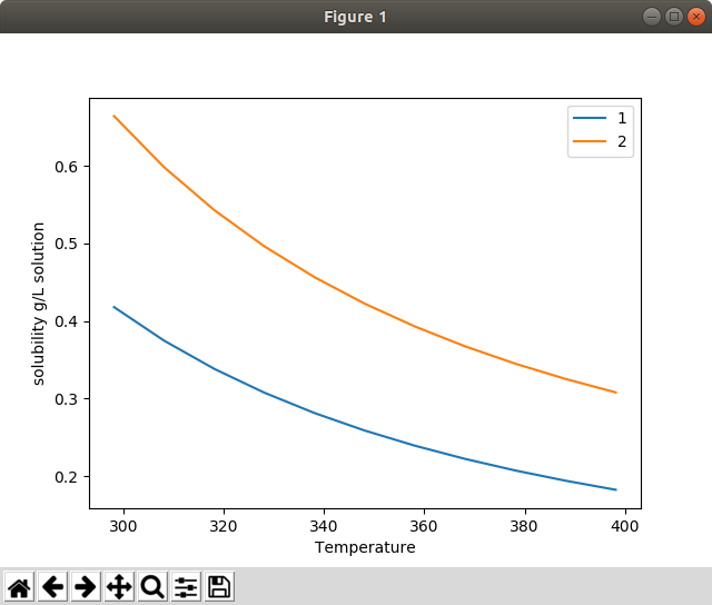
Fig. 3 The output of the plot function for a gas solubility calculation.
Examples
Partition coefficient
In this example, we calculate the logP of Ibuprofen. We use the standard octanol/water system. The code is as follows:
from scm.plams import *
from os import path

##################  Be sure to add the path to your own ADFCRS directory here  ##################
#################################################################################################
database_path = "<Path to ADFCRS directory containing .coskf files>"
#################################################################################################

if not path.exists(database_path):
    raise OSError(f'The provided path does not exist. Exiting.')

# initialize settings object
settings = Settings()
settings.input.property._h = 'LOGP'

# set the number of compounds
num_compounds = 3

compounds = [Settings() for i in range(num_compounds)]
compounds[0]._h = path.join( database_path, "1-Octanol.coskf" )
compounds[1]._h = path.join( database_path, "Water.coskf" )
compounds[2]._h = path.join( database_path, "Ibuprofen.coskf" )

#phase1 (octanol phase)
compounds[0].frac1 = 0.725
compounds[1].frac1 = 0.275

#phase2 (water phase)
compounds[0].frac2 = 0
compounds[1].frac2 = 1

#set temperature (range)
#to specify a range, use 3 numbers: (1) the lowest temperature,
#(2) the highest temperature, and (3) the steps taken between these temperatures
settings.input.temperature = "298.15"

# specify the compounds as the compounds to be used in the calculation
settings.input.compound = compounds
# create a job that can be run by COSMO-RS
my_job = CRSJob(settings=settings)
# run the job
init()
out = my_job.run()
finish()

# convert all the results into a python dict
res = out.get_results()

# print the logP of Ibuprofen
print ("logP of Ibuprofen:", res["logp"][2])
This generates the following output:
logP of Ibuprofen: [ 4.67381309]
Binary mixture
In this example, we calculate a binary mixture of water and 2-Hexanone and plot the vapor pressures as a function of composition. We also show how to change the method and calculate the binary mixture with the COSMO-SAC2013-Xiong model.
from scm.plams import *
from os import path

##################  Be sure to add the path to your own ADFCRS directory here  ##################
#################################################################################################
database_path = "<Path to ADFCRS directory containing .coskf files>"
#################################################################################################

if not path.exists(database_path):
    raise OSError(f'The provided path does not exist. Exiting.')

# initialize settings object
settings = Settings()
settings.input.property._h = 'BINMIXCOEF'

# let's also change to the COSMOSAC2013 method
settings.input.method = 'COSMOSAC2013'

# set the number of compounds
num_compounds = 2

compounds = [Settings() for i in range(num_compounds)]
compounds[0]._h = path.join( database_path, "Water.coskf" )
compounds[1]._h = path.join( database_path, "2-Hexanone.coskf" )

# use the vapor pressures from the VPM1 model
compounds[0].vp_equation = "VPM1"
compounds[0].vp_params = "-6093.40215895 -3.09584608667 0.000498622924643 34.47450247140318 0.0"
compounds[1].vp_equation = "VPM1"
compounds[1].vp_params = "-6474.348470271438 -6.057589837807771 0.003390587477679571 51.07134238467479 0.0"

#set temperature (range)
#to specify a range, use 3 numbers: (1) the lowest temperature,
#(2) the highest temperature, and (3) the steps taken between these temperatures
settings.input.temperature = "298.15"

# specify the compounds as the compounds to be used in the calculation
settings.input.compound = compounds
# create a job that can be run by COSMO-RS
my_job = CRSJob(settings=settings)
# run the job
init()
out = my_job.run()
finish()

# convert all the results into a python dict
res = out.get_results()

#plot all the pressures as a function of mole fraction of water
out.plot( "vapor pressure", "pressure", x_axis = res["molar fraction"][0], x_label="mole fraction water", y_label = "Pressure (bar)")
The code generates the following plot:
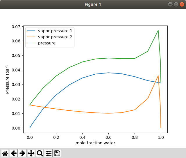
Fig. 4 A plot showing the total and partial vapor pressures for the water/2-Hexanone system.