PES point properties
No matter what application the AMS driver is used for, in one way or another it
always explores the potential energy surface (PES) of the system. One can
furthermore ask AMS to calculate additional properties of the PES in the points
that are visited. These are mostly derivatives of the energy, e.g. we can ask
AMS to calculate the gradients or the Hessian in the visited points. In general
all these PES point properties are requested through the Properties block in
the AMS input:
Properties
   Gradients [True | False]
   StressTensor [True | False]
   Hessian [True | False]
   SelectedAtomsForHessian integer_list
   NormalModes [True | False]
   ElasticTensor [True | False]
   Phonons [True | False]
End
This page in the AMS manual describes all the supported properties.
Note that because these properties are tied to a particular point on the potential energy surface, they are found on the engine output files. Note also that the properties are not always calculated in every PES point that the AMS driver visits during a calculation. By default they are only calculated in special PES points, where the definition of special depends on the task AMS is performing: For a geometry optimization properties would for example only be calculated at the final, converged geometry. This behaviour can often be modified by keywords special to the particular running task.
Nuclear gradients and stress tensor
The first derivative with respect to the nuclear coordinates can be requested as follows:
Properties
   Gradients [True | False]
End
PropertiesGradientsType: Bool Default value: False Description: Whether or not to calculate the gradients.
Note that these are gradients, not forces, the difference being the sign. The
gradients are printed in the output and written to the engine result
file belonging to the particular point on the PES in the
AMSResults%Gradients variable as a \(3 \times n_\mathrm{atoms}\) array
in atomic units (Hartree/Bohr).
For periodic systems (chains, slabs, bulk) one can also request the clamped-ion stress tensor (note: the clamped-ion stress is only part of the true stress tensor):
Properties
   StressTensor [True | False]
End
PropertiesStressTensorType: Bool Default value: False Description: Whether or not to calculate the stress tensor.
The clamped-ion stress tensor \(\sigma_\alpha\) (Voigt notation) is computed via numerical differentiation of the energy \(E\) WRT a strain deformations \(\epsilon_\alpha\) keeping the atomic fractional coordinates constant:
where \(V_0\) is the volume of the unit cell (for 2D periodic system \(V_0\) is the area of the unit cell, and for 1D periodic system \(V_0\) is the lenght of the unit cell).
The clamped-ion stress tensor (in Cartesian notation) is written to the engine
result file in AMSResults%StressTensor.
Hessian and normal modes of vibration
The calculation of the second derivative of the total energy with respect to the nuclear coordinates is enabled by:
Properties
   Hessian [True | False]
End
PropertiesHessianType: Bool Default value: False Description: Whether or not to calculate the Hessian.
The Hessian is not printed to the text output, but is saved in the engine result
file as variable AMSResults%Hessian. Note that this ist just the plain
second derivative (no mass-weighting) of the total energy and that for the order
of its \(3 \times n_\mathrm{atoms}\) columns/rows, the component index
increases the quickest: The first column refers to changes in the
\(x\)-component of atom 1, the second to the \(y\)-component, the
fourth to the \(x\)-component of the second atoms, and so on.
It is also possible to request the calculation of the normal modes of vibration:
Properties
   NormalModes [True | False]
End
PropertiesNormalModesType: Bool Default value: False Description: Whether or not to calculate the normal modes of vibration (and of molecules the corresponding Ir intensities.)
Note
For more information and advanced methods of calculating and analyzing molecular vibrations, see the manual chapter on the vibrational analysis (mode scanning, refinement and tracking).
This implies the calculation of the Hessian, which is required for calculating
normal modes. For engines that are capable of calculating dipole moments, this
also enables the calculation of the infrared intensities, so that the IR
spectrum can be visualized by opening the engine result file with ADFSpectra.
The normal modes of vibration and the IR intensities are saved to the
engine result file in the Vibrations section.
Note
The calculation of the normal modes of vibration needs to be done the
system’s equilibrium geometry. So one should either run the normal modes
calculation using an already optimized geometry, or combine both steps into
one job by using the geometry optimization task
together with the Properties%NormalModes keyword.
Symmetry labels of the normal modes of molecules may be calculated if AMS uses symmetry in the calculation of normal modes (key NormalModes%UseSymmetry).
If symmetry is used the nomal modes are projected against symmtric displacements for each irrep. If that is not successful the symmetric label is ‘MIX’.
Symmetry is only recognized if the starting geometry has symmetry.
Symmetry is only used for molecules if the molecule has a specific orientation in space, like that the z-axis is the main rotation axis.
If the GUI is used one can click the Symmetrize button (the star), such that the GUI will (try to) symmetrize and reorient the molecule.
There are some cases that even after such symmetrization, the orientation of the molecule is not what is needed for the symmetry to be used.
If that is the case or if key NormalModes%UseSymmetry is set to ‘False’ or if there is no symmetry, then no symmetry labels will be calculated.
NormalModes
   UseSymmetry [True | False]
End
NormalModesType: Block Description: Configures details of a normal modes calculation. UseSymmetryType: Bool Default value: True Description: Whether or not to exploit the symmetry of the system in the normal modes calculation.
Thermodynamics (ideal gas)
The following thermodynamic properties are calculated by default whenever normal modes are computed: entropy, internal energy, constant volume heat capacity, enthalpy and Gibbs free energy. Translational, rotational and vibrational contributions are calculated for entropy, internal energy and constant volume heat capacity. Moments of Inertia and principal axis of the system are also computed. These results are written to the output file (section: “Statistical Thermal Analysis”) and to the engine binary results file (section: “Thermodynamics”).
The thermodynamic properties are computed assuming an ideal gas, and electronic contributions are ignored. The latter is a serious omission if the electronic configuration is (almost) degenerate, but the effect is small whenever the energy difference with the next state is large compared to the vibrational frequencies. The thermal analysis is based on the temperature dependent partition function. The energy of a (non-linear) molecule is (if the energy is measured from the zero-point energy)
The summation is over all harmonic \(\nu_j\), \(h\) is Planck’s constant and \(D\) is the dissociation energy
Contributions from low (less than 20 1/cm) frequencies to entropy, heat capacity and internal energy are excluded from the total values, but they are listed separately (so the user can add them if they wish).
Thermo
   Pressure float
   TMax float
   TMin float
   nSteps integer
End
ThermoType: Block Description: Options for thermodynamic properties (assuming an ideal gas). The properties are computed for ‘nSteps’ temperatures in the range [TMin,TMax]. PressureType: Float Default value: 1.0 Unit: atm Description: The pressure at which the thermodynamic properties are computed. TMaxType: Float Default value: 298.15 Unit: Kelvin Description: Maximum value for the temperature range. TMinType: Float Default value: 298.15 Unit: Kelvin Description: Minimum value for the temperature range. nStepsType: Integer Default value: 1 Description: The number of temperatures in the range [TMin,TMax].
Partial Vibrational Spectra (PVDOS)
The Partial Vibrational Spectra (also known as PVDOS) is computed by default whenever normal modes are requested. The PVDOS \(P_{I,n}\) for atom \(I\) and normal mode \(n\) is defined as:
where \(m_I\) is the nuclear weight of atom \(I\), and \(\vec{\eta}_{I,n}\) is the diplacement vector for atom \(I\) in normal normal mode \(n\).
Tip
The Partial Vibrational Spectra (PVDOS) can be visualized using the ADFSpectra GUI module (Vibrations → Partial Vibrational Spectra (PVDOS)). When plotting a partial vibrational spectrum, the IR intensity of normal modes is scaled by the corresponding PVDOS of the selected atoms.
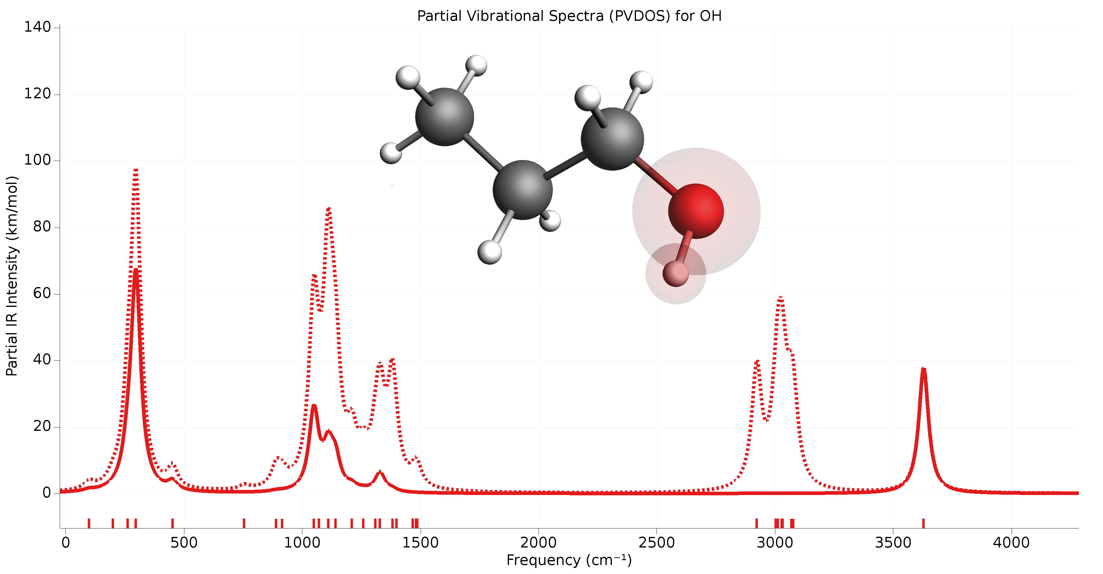
Fig. 1 Example of partial vibrational spectrum (PVDOS). The dotted line is the full IR spectrum of 1-propanol. The solid line is the PVDOS-scaled IR spectrum of the OH group (IR spectrum computed using GFN1-xTB).
The PVDOS matrix is not printed to the text output, but only saved to the engine
binary output (.rkf) in the variable Vibrations%PVDOS.
Elastic tensor
The elastic tensor \(c_{\alpha, \beta}\) (Voigt notation) is computed via second order numerical differentiation of the energy \(E\) WRT strain deformations \(\epsilon_\alpha\) and \(\epsilon_\beta\):
where \(V_0\) is the volume of the unit cell (for 2D periodic system \(V_0\) is the area of the unit cell, and for 1D periodic system \(V_0\) is the lenght of the unit cell).
For each strain deformation \(\epsilon_\alpha \epsilon_\beta\), the atomic positions will be optimized. The elastic tensor can be computed for any periodicity, i.e. 1D, 2D and 3D.
See also
To compute the elastic tensor, request it in the Properties input block of
AMS:
Properties
   ElasticTensor [True | False]
End
Note
The elastic tensor should be computed at the fully optimized geometry. One should therefore perform a geometry optimization of all degrees of freedom, including the lattice vectors. It is recommended to use a tight gradient convergence threshold for the geometry optimization (e.g. 1.0E-4). Note that all this can be done in one job by combining the geometry optimization task with the elastic tensor calculation.
The elastic tensor (in Voigt notation) is printed to the output file and stored
in the engine result file in the AMSResults
section (for 3D system, the elastic tensor in Voigt notation is a 6x6 matrix;
for 2D systems is a 3x3 matrix; for 1D systems is just one number).
Options for the numerical differentiation procedure can be specified in the
ElasticTensor input block:
ElasticTensor
   MaxGradientForGeoOpt float
   Parallel
      nCoresPerGroup integer
      nGroups integer
      nNodesPerGroup integer
   End
   StrainStepSize float
End
ElasticTensorType: Block Description: Options for numerical evaluation of the elastic tensor. MaxGradientForGeoOptType: Float Default value: 0.0001 Unit: Hartree/Angstrom Description: Maximum nuclear gradient for the relaxation of the internal degrees of freedom of strained systems. ParallelType: Block Description: The evaluation of the elastic tensor via numerical differentiation is an embarrassingly parallel problem. Double parallelization allows to split the available processor cores into groups working through all the available tasks in parallel, resulting in a better parallel performance. The keys in this block determine how to split the available processor cores into groups working in parallel. nCoresPerGroupType: Integer Description: Number of cores in each working group. nGroupsType: Integer Description: Total number of processor groups. This is the number of tasks that will be executed in parallel. nNodesPerGroupType: Integer Description: Number of nodes in each group. This option should only be used on homogeneous compute clusters, where all used compute nodes have the same number of processor cores.
StrainStepSizeType: Float Default value: 0.001 Description: Step size (relative) of strain deformations used for computing the elastic tensor numerically.
Phonons
Collective oscillations of atoms around theirs equilibrium positions, giving rise to lattice vibrations, are called phonons. AMS can calculate phonon dispersion curves within standard harmonic theory, implemented with a finite difference method. Within the harmonic approximation we can calculate the partition function and therefore thermodynamic properties, such as the specific heat and the free energy.
See also
Example: Phonons for graphene, Example: Phonons with isotopes and diamond lattice optimization and phonons tutorial
The calculation of phonons is enabled in the Properties block.
Properties
   Phonons [True | False]
End
Note
Phonon calculations should be performed on optimized geometries, including the lattice vectors. This can be done by either reading an already optimized system as input, or combining the phonon calculation with the geometry optimization task.
The details of the phonon calculations are configured in the
NumericalPhonons block:
NumericalPhonons
   SuperCell # Non-standard block. See details.
      ...
   End
   StepSize float
   DoubleSided [True | False]
   UseSymmetry [True | False]
   Interpolation integer
   NDosEnergies integer
   Parallel
      nCoresPerGroup integer
      nGroups integer
      nNodesPerGroup integer
   End
End
NumericalPhononsSuperCellType: Non-standard block Description: Used for the phonon run. The super lattice is expressed in the lattice vectors. Most people will find a diagonal matrix easiest to understand.
The most important setting here is the super cell transformation. In principle this should be as large as possible, as the phonon bandstructure converges with the size of the super cell. In practice one may want to start with a 2x2x2 cell and increase the size of the super cell until the phonon band structure converges:
NumericalPhonons
   SuperCell
      2 0 0
      0 2 0
      0 0 2
   End
End
Other keywords in the NumericalPhonons block modify the details of the numerical differentiation
procedure and the accuracy of the results:
NumericalPhononsStepSizeType: Float Default value: 0.04 Unit: Angstrom Description: Step size to be taken to obtain the force constants (second derivative) from the analytical gradients numerically. DoubleSidedType: Bool Default value: True Description: By default a two-sided (or quadratic) numerical differentiation of the nuclear gradients is used. Using a single-sided (or linear) numerical differentiation is computationally faster but much less accurate. Note: In older versions of the program only the single-sided option was available. UseSymmetryType: Bool Default value: True Description: Whether or not to exploit the symmetry of the system in the phonon calculation. InterpolationType: Integer Default value: 100 Description: Use interpolation to generate smooth phonon plots. NDosEnergiesType: Integer Default value: 1000 Description: Nr. of energies used to calculate the phonon DOS used to integrate thermodynamic properties. For fast compute engines this may become time limiting and smaller values can be tried.
Note that the numerical phonon calculation supports AMS’ double
parallelism, which can perform the calculations for the
individual displacements in parallel. This is disabled by default but can be
enabled using the keys in the NumericalPhonons%Parallel block:
NumericalPhononsParallelType: Block Description: Computing the phonons via numerical differentiation is an embarrassingly parallel problem. Double parallelization allows to split the available processor cores into groups working through all the available tasks in parallel, resulting in a better parallel performance. The keys in this block determine how to split the available processor cores into groups working in parallel. Keep in mind that the displacements for a phonon calculation are done on a super-cell system, so that every task requires more memory than the central point calculated using the primitive cell. nCoresPerGroupType: Integer Description: Number of cores in each working group. nGroupsType: Integer Description: Total number of processor groups. This is the number of tasks that will be executed in parallel. nNodesPerGroupType: Integer Description: Number of nodes in each group. This option should only be used on homogeneous compute clusters, where all used compute nodes have the same number of processor cores.
Numerical differentiation options
The following options apply whenever AMS computes gradients, hessians or stress tensors via numerical differentiation.
NumericalDifferentiation
   NuclearStepSize float
   Parallel
      nCoresPerGroup integer
      nGroups integer
      nNodesPerGroup integer
   End
   StrainStepSize float
   UseSymmetry [True | False]
End
NumericalDifferentiationType: Block Description: Define options for numerical differentiations, that is the numerical calculation of gradients, Hessian and the stress tensor for periodic systems. NuclearStepSizeType: Float Default value: 0.005 Unit: Bohr Description: Step size for numerical nuclear gradient calculation. ParallelType: Block Description: Numerical differentiation is an embarrassingly parallel problem. Double parallelization allows to split the available processor cores into groups working through all the available tasks in parallel, resulting in a better parallel performance. The keys in this block determine how to split the available processor cores into groups working in parallel. nCoresPerGroupType: Integer Description: Number of cores in each working group. nGroupsType: Integer Description: Total number of processor groups. This is the number of tasks that will be executed in parallel. nNodesPerGroupType: Integer Description: Number of nodes in each group. This option should only be used on homogeneous compute clusters, where all used compute nodes have the same number of processor cores.
StrainStepSizeType: Float Default value: 0.001 Description: Step size (relative) for numerical stress tensor calculation. UseSymmetryType: Bool Default value: True Description: Whether or not to exploit the symmetry of the system for numerical differentiations.
Note that the numerical differentiation calculation supports AMS’ double
parallelism, which can perform the calculations for the
individual displacements in parallel. This is disabled by default but can be
enabled using the keys in the NumericalDifferentiation%Parallel block.
AMS may use symmetry (key NumericalDifferentiation%UseSymmetry) in case of numerical differentiation calculations.
If symmetry is used only symmetry unique atoms are displaced.
Symmetry is only recognized if the starting geometry has symmetry.
Symmetry is only used for molecules if the molecule has a specific orientation in space, like that the z-axis is the main rotation axis.
If the GUI is used one can click the Symmetrize button (the star), such that the GUI will (try to) symmetrize and reorient the molecule.
There are some cases that even after such symmetrization, the orientation of the molecule is not what is needed for the symmetry to be used in case of numerical differentiation calculations. If that is the case or if key NumericalDifferentiation%UseSymmetry is set to ‘False’, then no symmetry will be used.