OLED workflows

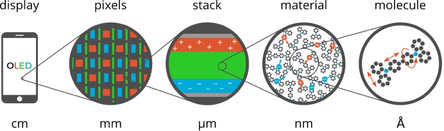
Starting with the 2022 release of the Amsterdam Modeling Suite we include a set of workflow scripts for multiscale OLED modeling. These workflows are developed and validated in close collaboration with Simbeyond to bridge the gap between ab-initio atomistic modeling of OLED molecules with AMS, and device level kinetic Monte Carlo simulations using Simbeyond’s Bumblebee code. Together with Simbeyond, we attempt to provide a fully integrated multiscale simulation platform for the digital screening and prediction of successful OLED materials and devices.

The Amsterdam Modeling Suite implements the atomistic simulation part of this multiscale toolchain in the form of two workflow scripts:

• Deposition

  The first step simulates the growth of a thin film in a molecular dynamics and force-bias Monte Carlo calculation mimicking physical vapor deposition.

• Properties

  In the second step the morphology resulting from the deposition is used to obtain the distributions (and possibly spatial correlations) of molecular properties such as ionization potential, electron affinity and exciton energies at the DFT level. Each molecule’s environment is taken into account in a polarizable QM/MM scheme using the DRF model.

The output of the Properties workflow is an HDF5 file containing a summary of the results for a material. This file can be opened in AMSview for a visualization of the results, but also directly imported into Simbeyond’s Bumblebee code to use it in simulations at the device level.

This manual page describes the technical details and options of the OLED workflow scripts. For a more hands-on introduction, you may want to start with the GUI tutorial, that will guide you through the entire workflow using the hole transport material β-NPB as an example.

See also

Tutorial on multiscale modeling of OLED devices

Note

The OLED workflow scripts use ADF and DFTB. In addition to the Advanced Workflows and Tools license, you will therefore also need a license for ADF and DFTB in order to use the OLED workflows.

Deposition

The deposition workflow implements a series of mixed molecular dynamics and force-bias Monte Carlo calculations to simulate the growth of a thin film with physical vapor deposition.

Deposition of mCP

The molecule gun is used to shoot molecules at the substrate. Upon reaching the surface, the force-bias Monte Carlo method is used to accelerate the search for favorable adsorption sites. This process is repeated until a thin film of a user-defined thickness has grown on the substrate.

To make this process computationally more efficient, the deposition happens in so called “cycles”. At the end of each deposition cycle, the bulk material at the bottom of the growing film is “trimmed off” and stored. Only the two top layers (each about 10 Å thick) are transferred to the next deposition cycle, where the lower of the two layers is frozen. This ensures that the trimmed off parts of the system fit perfectly together when the system is reassembled in the end of the simulation. By depositing in cycles we avoid simulating a lot of bulk material and are able to make the total computational cost linear in the thickness of the deposited film.

At the end of the simulation the layer deposited by the individual cycles are stacked and a short molecular dynamics calculation on the entire film is used to anneal it from the deposition temperature down to 300K at ambient pressure.

An entire deposition with 6 deposition cycles (and the final equilibration to room temperature) is shown in the video on the right.

Basic input

The minimal input to the deposition workflow just specifies what to deposit:

#!/bin/sh

DEPOSITION_JOBNAME=myDeposition $AMSBIN/oled-deposition << EOF

Molecule
   SystemName myMol
End

System myMol
   ...
End

EOF

The Molecule block is only really used when depositing mixed molecule materials, e.g. host-guest systems. This will be explained in a separate section below. For a single molecule deposition there should just be one Molecule block that references the only System block by name via the SystemName keyword, as shown in the example above.

The System block used by the OLED deposition script closely follows the System block in the input for the AMS driver, but supports only a subset of the keywords:

System

Type:Block Recurring:True Description:Specification of the chemical system. For some applications more than one system may be present in the input. In this case, all systems except one must have a non-empty string ID specified after the System keyword. The system without an ID is considered the main one.

Atoms

Type:Non-standard block Description:The atom types and coordinates. Unit can be specified in the header. Default unit is Angstrom.

GeometryFile

Type:String Description:Read the geometry from a file (instead of from Atoms and Lattice blocks). Supported formats: .xyz

BondOrders

Type:Non-standard block Description:Defined bond orders. Each line should contain two atom indices, followed by the bond order (1, 1.5, 2, 3 for single, aromatic, double and triple bonds) and (optionally) the cell shifts for periodic systems. May be used by MM engines and for defining constraints. If the system is periodic and none of the bonds have the cell shift defined then AMS will attempt to determine them following the minimum image convention.

Just like in the AMS driver, as an alternative to the System block, you an also use the LoadSystem block to load a system directly from a .rkf file of a previous calculation.

The deposition workflow uses the ForceField engine for the molecular dynamics simulation of the physical vapor deposition. In order to also support the deposition of metal containing compounds, we use the UFF force field with the UFF4MOF-II parametrization for the deposition. As with any calculation with the ForceField engine you may manually provide (UFF4MOF-II) atom-types, atomic charges and bond orders in the input file:

System
  Atoms
     C  [...]  ForceField.Type=C_R  ForceField.Charge=-0.1186
     N  [...]  ForceField.Type=N_R  ForceField.Charge=-0.2563
     H  [...]  ForceField.Type=H_   ForceField.Charge=+0.1021
     [...]
  End
  BondOrders
     1 2 1.0
     1 5 1.5
     1 6 1.5
     [...]
  End
End

Whatever is not specified in the input will automatically be determined: the input system is optimized with ADF using the S12g exchange-correlation functional with a TZP basis set. At the optimized geometry, the Charge Model 5 is used to calculate the atomic charges, while the rounded Nalewajski-Mrozek bond orders determine the topology. See the ADF manual for details on the calculation of charges and bond orders. Finally, using the topology determined by the calculated bond orders, the automatic UFF atom-typing that is built into the ForceField engine is used to determine the atom-types.

If you want to make sure the correct atom-types and bonds are used in your calculation, we recommend building the system in AMSinput, where you can visually check the bond orders and atom-types to make sure they are correct. The result can then be exported into a file as a System block via File → Export coordinates → .in. For the atomic charges we recommend relying on the automatic calculation with ADF. (Just make sure the ForceField.Charge suffixes are not included in the atom block. Their absence will trigger the automatic charge calculation with ADF.)

By default a box of 60 x 60 x 120 Å is deposited. The first two dimensions give the surface area of the deposited layer, while the third dimension is the thickness of the layer. The size of the deposited box can be changed using the Size keyword in the Box block:

Box
   Size 60 60 120
End

Box

Type:Block Description:Specifications of the box into which the material is deposited.

Size

Type:Float List Default value:[60.0, 60.0, 120.0] Unit:Angstrom GUI name:Box size Description:Specify the desired size of the box. The final deposited box may have a different size. The x- and y-axis are perpendicular to the direction of deposition, so these may be regarded as the width of the growing layer. The z-axis is the direction along which the deposition happens, so this determines the thickness of the deposited layer. Note that the x- and y-axis will be ignored if a custom substrate is used: the are of the box is then determined by the lattice of the substrate. The z-axis can still be freely chosen, but should be large enough that there is enough space for the substrate itself and to deposit more molecules on top of it.

With sizes typical for molecules used in OLED devices, the default box size results in a deposition of ~500 molecules. Note that the computational time of a deposition scales linearly with the thickness of the layer, but quadratically with the surface area. This is because a larger area requires both the deposition of more molecules to fill the box, but also makes each MD step more expensive as more molecules have to be simulated at the same time. When increasing the thickness of the layer, molecules at the bottom are first frozen, and later removed from the simulation altogether, giving an overall linear scaling.

The temperature at which the deposition is performed can be configured in the Deposition section.

Deposition
   Temperature float
End

Deposition

Type:Block Description:Specifies the details of how molecules are deposited.

Temperature

Type:Float Default value:600.0 Description:The temperature at which the deposition happens.

Finally, there are a couple more technical options in the Deposition section, that we suggest to leave at their default values.

Deposition
   Frequency integer
   TimeStep float
   ConstrainHXBonds Yes/No
   NumMolecules integer
End

Deposition

Type:Block Description:Specifies the details of how molecules are deposited.

Frequency

Type:Integer Default value:10000 Description:The frequency in MD steps at which new molecules will be added to the system.

TimeStep

Type:Float Default value:1.0 Unit:Femtoseconds Description:The time difference per step.

ConstrainHXBonds

Type:Bool Default value:Yes GUI name:Constrain H-* bonds Description:Constrain the bond length for all H-* bonds (i.e. any bond to a hydrogen atom). Doing this allows choosing a larger time step. If this option is disabled, the TimeStep needs to be reduced manually.

NumMolecules

Type:Integer Description:The number of molecules that we will try to deposit. If not specified the number will be determined automatically such that the box becomes approximately full.

Output

Running the oled-deposition workflow script creates a single directory in which you can find all results of a deposition. By default this directory is named deposition.workdir, but in order to avoid name clashes, that location can be changed with the DEPOSITION_WORKDIR environment variable, similar to AMS_JOBNAME for the AMS driver. The example below will collect all results in the directory myMol.workdir:

#!/bin/sh

DEPOSITION_WORKDIR=myMol $AMSBIN/oled-deposition << EOF
...
EOF

Let us go through all files and folders in the working directory in the order in which they are created.

Firstly, the working directory contains a logfile. The contents of the logfile are identical to what you see on standard output when running the oled-deposition workflow.

The deposition workflow starts with a couple of calculations on single molecules in vacuum. Each of them runs in a separate folder, in which you can find the usual AMS output files (such as ams.rkf):

dft_opt/
ff_opt/
equilibrate_ff_input_molecule/

The dft_opt directory contains the results of the initial geometry optimization with ADF, which is used to determine the atomic charges and bond orders if these were not specified in the input. The ff_opt directory contains the results of a subsequent geometry optimization using the ForceField engine with the UFF4MOF-II forcefield. In this step the atom-types are determined if they were not specified in the input already. Finally in the equilibrate_ff_input_molecule directory a short MD simulation at the deposition temperature is performed to equilibrate the molecule to the desired temperature. We suggest visualizing the trajectory of this equilibration in AMSmovie to make sure the molecule does not undergo unexpected conformational changes that could be caused by wrong atom-types or bonds. If the molecule behaves strangely (or falls apart) at this point, one may need to go back and assign atom-types and bonds manually in the input.

When depositing mixtures you will see multiple instances of the three directories above: one for each deposited species.

Once all the preparatory work is done, the actual deposition cycles each write a folder and (upon completion of the cycle) two files:

depo_cycle_1/
depo_box.1.in
depo_box.1.xyz

You can follow the progress of your deposition by opening the ams.rkf in the last depo_cycle_*/ directory. The depo_box.*.in and depo_box.*.xyz files contain the entire morphology deposited so far: by visualizing them in order you can watch your material grow!

Important

The files with the .in extension contain the System geometry in form of a System block. This format contains bond orders, force field atom-types as well as atomic charges. It can be opened in AMSinput and PLAMS and should be the preferred format when working with the OLED workflow scripts in AMS. The .xyz file is in extended XYZ format does not contain that extra information. Always use a .in file when transferring a system from one script to the next, e.g. when going from the OLED deposition to the OLED properties workflow.

Once all molecules have been deposited the entire box is annealed from the deposition temperature down to room temperature. This creates one directory and (upon completion) a .in and .xyz file containing the annealed morphologies:

equilibrate_box/
equil_box.in
equil_box.xyz

The last step is to take the room temperature morphology and perform a geometry optimization on it. This essentially removes all thermal vibrations and results in a geometry that is relaxed at the force field level. As you might expect, the last step also produces a folder and (upon completion) a .in and .xyz file:

optimize_box/
opt_box.in
opt_box.xyz

It is up to the user to decide whether to continue to the OLED properties workflow with the morphology from equil_box.in (equilibrated to 300K) or opt_box.in file (fully relaxed). (We recommend using the fully relaxed morphology though.)

Deposition of host-guest materials

A deposition of host-guest materials can easily be done by specifying multiple Molecule and System blocks in the input. The following runscript generates a 95% to 5% mixture (by number of molecules) of two compounds:

#!/bin/sh

DEPOSITION_JOBNAME=host_guest $AMSBIN/oled-deposition << EOF

Molecule
   SystemName myHost
   MoleFraction 0.95
End
Molecule
   SystemName myGuest
   MoleFraction 0.05
End

System myHost
   ...
End
System myGuest
   ...
End

EOF

Molecule
   MoleFraction float
   SystemName string
End

Molecule

Type:Block Recurring:True GUI name:Molecules Description:Specification of the molecule to be deposited.

MoleFraction

Type:Float Default value:1.0 GUI name:Molar fraction Description:The relative occurrence of the molecule with regard to other deposited species. Only relevant for mixed molecule depositions.

SystemName

Type:String GUI name:Molecule Description:String ID of a named [System] to be inserted. The lattice specified with this System, if any, is ignored and the main system’s lattice is used instead.

You can have an arbitrary number of Molecule blocks in your input to deposit multi-component mixtures. Obviously, the box your are depositing must be large enough that it still contains at least a few molecules of the rarest component.

Note that multiple Molecule and System blocks can also be used to deposit different conformers of the same compound. While conformational changes can in principle happen over the course of the MD simulation, it may be a good idea to deposit a mixture of conformers directly if their geometries are very different.

Deposition of interfaces

By default the deposition will use a single graphene layer as a substrate. The graphene layer is removed after the first deposition cycle and will not be included in the output morphologies, i.e. the .in files in the working directory. Note that the graphene layer is not present in the annealing of the entire morphology from deposition temperature to 300K, which is performed at the end of the workflow. The result of this is that both the bottom and top of the deposited thin-film by default represents an interface between the material and a vacuum.

Instead of depositing on a clean graphene sheet, the deposition workflow also supports custom substrates. This is intended to be used for depositing a thin film of one material on top of another material and allows users to study the interface between the two. A custom substrate is set up using the Substrate and SubstrateSystem keys in the Box block.

Box
   Substrate [Graphene | Custom]
   SubstrateSystem string
End

Box

Type:Block Description:Specifications of the box into which the material is deposited.

Substrate

Type:Multiple Choice Default value:Graphene Options:[Graphene, Custom] Description:The substrate on which to grow the layer.

SubstrateSystem

Type:String GUI name:Custom substrate Description:String ID of a named [System] to be used as a substrate. (This is only used when the Substrate key is set to Custom.)

Here the value of the SubstrateSystem refers to a named System block in the input, representing the geometry of the substrate. The following example shows how to deposit a molecule B on top of a substrate of molecule A:

#!/bin/sh

DEPOSITION_JOBNAME=molB_on_molA $AMSBIN/oled-deposition << EOF

Molecule
   SystemName molB
End
System molB
   ...
End

Box
   Size 0 0 240
   Substrate Custom
   SubstrateSystem molA_substrate
End

System molA_substrate
   Atoms
      ...
   End
   BondOrders
      ...
   End
   Lattice
      ...
   End
End

EOF

The contents of the block System molA_substrate should be obtained by first running a deposition of molecule A: just use the System block found in e.g. the equil_box.in file of that deposition as the custom substrate for the next job. (Note that no attempt will be made to automatically determine atomic charges, bond orders, or force-field atom types for the molecules in the substrate. Taking the System block from the results of an earlier deposition is the easiest way ensure you are using exactly the same bonds, atom types and charges for the substrate molecules in the new calculation.)

Warning

The custom substrate option can currently not be used to deposit thin films on top of crystalline materials. The substrate must consist of individual molecules and be >20 Å thick, so that it can be split into a frozen (lower) and thermostatted (upper) layers.

Note that the Box%Size in the x- and y-direction is ignored when using a custom substrate: the size of the custom substrate is used instead. The thickness of the layer can be set manually when using a custom substrate, but it needs to accommodate both the already existing substrate as well as the newly grown film on top. Assume that the thickness of the substrate film is 120 Å in the example above. By setting the the z-value of the Box%Size to 240 Å, we will have space to accommodate the substrate and then grow another layer of 120 Å thickness on top of it. Note that while the default graphene layer is removed from the morphology, a custom substrate will be included in the morphology.

Restarting a deposition

The OLED workflow scripts are based on the PLAMS scripting framework. As such it can rely on the PLAMS rerun prevention to implement restarting of interrupted depositions.

The easiest way to restart a deposition is to include the --restart (or short: -r) command line flag:

#!/bin/sh

DEPOSITION_JOBNAME=myDeposition $AMSBIN/oled-deposition --restart << EOF
...
EOF

This first (interrupted) run will have created the myDeposition.workdir directory. Running the above script again will move that directory to myDeposition.workdir.res and reuse all successful jobs from the first run. (People already familiar with PLAMS will recognize that this works just like the -r flag on the PLAMS launch script.) Note that this does not restart the previous deposition precisely at the point where it was interrupted. Instead it restarts from the beginning of the last deposition cycle.

When running a deposition workflow on a batch system such as SLURM, you may want to consider always including the --restart flag in your runscript. It is not a problem if there are no previous results to restart from, but in case your job gets interrupted and automatically rescheduled, the --restart flag will make sure that it continues (approximately) where it stopped.

There is also the RestartWorkdir keyword in the input file:

#!/bin/sh

DEPOSITION_JOBNAME=newDepo $AMSBIN/oled-deposition << EOF

RestartWorkdir oldDepo.workdir

...

EOF

RestartWorkdir

Type:String Description:Uses the data from the working directory of a previously run deposition workflow for restarting. Under the hood this uses the normal rerun-prevention available in PLAMS: it may reuse results from old jobs instead of running them again.

While this can be used to accomplish the same thing the --restart flag would do, its best use is to specify a RestartWorkdir of a previous deposition of the same molecules. This can save you the initial step of doing the DFT calculations in order to determine the atomic charges and bonds. A perfect use it when you have already deposited a mixture, and later decide to change the ratio between the compounds: by specifying the working directory of the first deposition the initial DFT calculations can be skipped entirely.

Properties

The properties workflow is used to obtain distributions (and possibly spatial correlations) of molecular properties such as ionization potential and electron affinity from the morphology. To accomplish this, it will perform DFT calculations on all individual molecules from the morphology, taking their environment into account in QM/MM calculation.

The exact workflow (with all default settings) is as follows:

1. For each molecule in the box, do a quick DFT calculation with LDA and a DZP basis and use the MDC-D charge model to determine atomic charges. These charges will be used for the electrostatic part of the embedding potential in the next step.

mCP in 15 Å environment

2. For each molecule in the box:
   • Determine which other molecules to consider as the environment. By default all molecules within 15 Å (atom-atom distance) are considered.

   • Individually, for neutral molecule, cation, and anion:

     • Optimize geometry of central QM molecule in frozen MM environment using GFN1-xTB and UFF4MOF-II with electrostatic embedding in the Hybrid engine.
     • Do a DFT single point on the optimized geometry using PBE and an all-electron TZ2P basis. The environment is taken into account using a polarizable DRF embedding. (For the neutral systems exciton energies and transition dipole moments are also computed with TD-DFT.)

   • Calculate the (approximately) adiabatic ionization potential and electron affinity from the differences in total energy with respect to the neutral system.
3. For all pairs of neighboring molecules (within 4 Å atom-atom distance of each other) calculate the electron and hole charge transfer integrals with GFN1-xTB.

What is described above is the workflow with all default settings. Various aspects of this (such as the ranges) can be tweaked from the input, see the Settings section below.

Warning

The calculation of exciton properties and transfer integrals is in a very early state. We have not verified their accuracy against experiment, and expect both the excitation energies as well as the transfer integrals to be severely underestimated in AMS2021.1. We will improve the calculation of exciton properties and transfer integrals in the future.

Basic input

The simplest possible input for the oled-properties workflow script is just a single System block.

#!/bin/sh

$AMSBIN/oled-properties << EOF

System
   Atoms
      ...
   End
   Lattice
      ...
   End
  [BondOrders
      ...
   End]
End

EOF

Obviously, the Atoms and Lattice blocks are required, while the BondOrders block is optional. If the bond orders are present, they will be used to determine which parts of the system are connected, which ultimately determines which sets of atoms are considered distinct molecules. If the BondOrders block is not present, the bonds will be guessed. Since we only care about which atoms are bonded at all, and not on details such as the bond order, this should work quite reliably.

Nevertheless, if the morphology was obtained with the AMS deposition workflow, we can use the fact that it writes out the morphology as a .in file containing exactly the System block we need. Basically, we use the System block from e.g. the opt_box.in output file of the deposition as the input for the properties script.

#!/bin/sh

$AMSBIN/oled-deposition << EOF
   ... see oled-deposition manual page ...
EOF

$AMSBIN/oled-properties < deposition.workdir/opt_box.in

This has the advantage that the bonds are guaranteed to be transferred without change between the two workflows.

Output

Working directory

Running the oled-properties workflow script creates a single directory in which you can find all results of the calculation. By default this directory is named properties.workdir, but in order to avoid name clashes, that location can be changed with the PROPERTIES_WORKDIR environment variable, similar to AMS_JOBNAME for the AMS driver. The example below will collect all results in the directory myMaterial.workdir:

#!/bin/sh

PROPERTIES_WORKDIR=myMaterial $AMSBIN/oled-properties << EOF
...
EOF

This will create the myMaterial.workdir directory with roughly the following internal structure:

myMaterial.workdir/
├── logfile
├── atomic_charges
│   ├── 0/
│   │   ├── adf.rkf
│   │   ├── ams.log
│   │   └── ...
│   ├── 1/
│   │   ├── adf.rkf
│   │   ├── ams.log
│   │   └── ...
│   └── .../
└── properties/
    ├── relax_0/
    │   ├── ams.rkf
    │   ├── ams.log
    │   └── ...
    ├── 0/
    │   ├── adf.rkf
    │   ├── ams.log
    │   └── ...
    ├── relax_0_-1/
    │   ├── ams.rkf
    │   ├── ams.log
    │   └── ...
    ├── 0_-1/
    │   ├── adf.rkf
    │   ├── ams.log
    │   └── ...
    ├── relax_0_1/
    │   ├── ams.rkf
    │   └── ...
    ├── 0_1/
    │   ├── adf.rkf
    │   ├── ams.log
    │   └── ...
    ├── .../
    └── summary.hdf5

The atomic_charges directory contains the results from the intial pass over all molecules, in which the atomic charges are determined with a quick DFT calculations. These charges are later be used for the electrostatic part of the embedding. The directory will be missing if you did not use DFT as the setting for the Embedding%Charges keyword.

The properties directory contains the results from the second pass over all molecules. The first number in the name of the subdirectories is again the ID of the molecule (starting from zero). This is followed by the total charge for the calculations on the ions. The QM/MM geometry optimizations used to obtain approximate equilibrium structures follow the same naming scheme, with the added relax_ prefix. If you choose not to relax (ion) geometries by setting the Relax keyword to None (or Neutral), the relax_* folders (or at least some of them) may be missing.

Data on the HDF5 file

I addition to the full output of all individual calculations, you will also get a small HDF5 file called summary.hdf5 containing a summary of the results of your calculations. These are generally just the results that are usually interesting for the design of OLED materials, such as site energies, exciton energies, (transition) dipole moments, etc. This file can be imported into Simbeyond’s Bumblebee code to use your calculated material in a device level kinetic Monte Carlo simulation. The following groups and datasets can be found on the HDF5 file. Note that all arrays on the HDF5 file are indexes starting from zero.

The species group contains information about the different molecular species making up the morphology. There are two arrays in the species group whose size is equal to the number of different species (numSpecies):

species.name

An array of human readable names identifying the molecular species making up the morphology. Currently this is just the molecular formula in Hill notation.

species.smiles

An array of SMILES strings for the different molecular species. May contain a dummy value in case the determination of the SMILES string from the 3D structure fails for a species.

The molecules group contains the complete geometrical description of the morphology. It contains a number of arrays, (almost) all of which have the total number of molecules (numMolecules) as their size:

molecules.species

An array of integers containing the species a molecule in for of an index into the arrays in the species group.

molecules.lattice

(3 x 3) array containing the lattice vectors in Ångstrom.

molecules.position

(numMolecules x 3) array containing the center of mass positions of all molecules in Ångstrom. Note that all center of mass positions are within the parallelepiped spanned by the lattice vectors, i.e. all fractional coordinates are in the [0,1] range.

molecules.atoms

This is an numMolecules sized 1D array, where each element itself is an array of string,float,float,float tuples representing symbol,x,y,z. The x, y and z coordinates are given in Ångstrom.

molecules.bonds

This is an numMolecules sized 1D array, where each element itself is an array of int,int,float tuples representing atom1,atom2,bondOrder. Here atom1 and atom2 are indices into the corresponding element of the molecules.atoms array. The bondOrder is a floating point number, where the value of 1.5 is used to represent an aromatic bond.

The site energies are contained in the energies group on the HDF5 file:

energies.IP

A numMolecules sized array containing the first ionization potential for each molecule in eV.

energies.EA

A numMolecules sized array containing the first electron affinity for each molecule in eV.

energies.HOMO

A numMolecules sized array containing the Kohn-Sham orbital energy of the highest occupied orbital in eV. If requested via the NumAdditionalEnergies keyword in the input of the properties workflow, more arrays of this type (HOMO-1, HOMO-2, …) may exist and contain the orbital energies of lower lying occupied orbitals.

energies.LUMO

A numMolecules sized array containing the Kohn-Sham orbital energy of the lowest unoccupied orbital in eV. If requested via the NumAdditionalEnergies keyword in the input of the properties workflow, more arrays of this type (LUMO+1, LUMO+2, …) may exist and contain the orbital energies of higher lying virtual orbitals.

Similarly the exciton energies (in eV) can be found in the exciton_energies group. If the calculation of exciton energies was disabled by setting NumExcitations to 0 in the input, this information is not present.

exciton_energies.S1

Energies of the first excited singlet state (S1) with respect to the ground state. Higher singlet excitation energies may be found in more arrays of this type (S2, S3, …) if their calculation was requested by setting NumExcitations to a value larger 1.

exciton_energies.T1

Energies of the first excited triplet state (T1) with respect to the ground state. Higher triplet excitation energies may be found in more arrays of this type (T2, T3, …) if their calculation was requested by setting NumExcitations to a value larger 1.

Static dipole moments and transition dipole moments (in Debye) can be found in their respective groups:

static_multipole_moments.dipole_moment

(numMolecules x 3) array containing the dipole moment vectors for each molecule.

transition_dipole_moments.S1_S0

(numMolecules x 3) array containing the transition dipole moment vectors for the S0 → S1 transition for each molecule. Transition dipole moments for higher singlet excitations may be found in more arrays of this type (S2_S0, S3_S0, …) if their calculation was requested by setting NumExcitations to a value larger 1.

If the calculation of transfer integrals is requested with the TransferIntegrals%Type key in the input, the pairs and transfer_integrals groups will also be available on the HDF5 file, containing the following datasets:

pairs.indices

A (numPairs x 2) array of integers containing the molecule indices for all pairs of molecules that were considered close enough to trigger the calculation of transfer integrals between them.

transfer_integrals.electron

A numPairs sized array containing the transfer integral (in eV) for electrons between each pair.

transfer_integrals.hole

A numPairs sized array containing the transfer integral (in eV) for holes between each pair.

Accessing the HDF5 file

The easiest way to view the data from the HDF5 file is to open it in the GUI using the AMSview module. There you can easily plot histograms of all the calculated properties, but also visualize the spacial distribution of the properties.

For more custom built analysis, the HDF5 file can easily be opened from Python using the h5py library, which is included in the AMS Python Stack. The following code snippet shows how to calculate the mean and standard deviation of the ionization potential:

import h5py

with h5py.File("summary.hdf5", "r") as f:
   IPs = f['energies']['IP'].value
   print("IP = ", IPs.mean(), "±" , IPs.std())

The above snippet is only suitable for calculations of pure compounds, as we are calculating the mean and standard deviation over all molecules, not taking their species into account. For mixtures calculating these properties per species would be much more useful. This can easily be accomplished by using an appropriate mask on the IPs array for the calculation of mean and standard deviation:

import h5py
import numpy as np

with h5py.File("summary.hdf5", "r") as f:
   IPs        = f['energies']['IP'].value
   speciesIDs = f['molecules']['species'].value

   for specID, specName in enumerate(f['species']['name']):
         mask = (speciesIDs==specID) & (~np.isnan(IPs))
         print(specName)
         print("IP = ", IPs[mask].mean(), "±" , IPs[mask].std())

Note how we also use the mask to exclude all NaN elements in the array from the calculation of the mean and standard deviation. Occasional NaN values in the arrays on the HDF5 file indicate that a property could not be calculated for a molecule because the job for it crashed or failed in some other way. This is not a problem as long as it happens only rarely, but the NaN values need to be excluded from the analysis.

Parallelization

As you can imagine, the properties workflow is computationally quite expensive. After all, we are doing hundreds of (TD-)DFT calculations on relatively large molecules. Luckily all the calculations on the different molecules are independent from each other, and can therefore run in parallel. The workflow scripts supports different methods of parallelization through the JobRunner keyword.

JobRunner

Type:String Default value:local:*,4 Description:Configures how the jobs will be executed. • local:N,M: Run the jobs locally. Here N is the number of jobs to run in parallel, and M is the number of CPU cores used by each job. The total number of CPU cores used will be the product of N and M. Note that N or M can be replaced by the asterisk as a wildcard. In that case the missing number will be automatically determined such that in total $NSCM CPU cores will be utilized. If $NSCM is not set, the entire machine will be utilized. • batch_system:submit_cmd: Submit the individual jobs to a batch system. Example: slurm:sbatch -p mars -N 1 -n 4 will submit each job with 4 tasks/cores on 1 node to the mars partition of a SLURM batch system. Please refer to the PLAMS GridRunner documentation for a list of supported batch systems.

Local job execution

The simplest option (local) is to run the job on the machine that also executes the workflow script itself. This is a good option if you have access to a powerful machine with many CPU cores, on which you can run jobs directly (i.e. not through a batch system). By default 4 cores will be used for the execution of each job, and enough jobs will be run in parallel to saturate the entire machine:

JobRunner local:*,4

See above for a detailed description of the local option.

Job submission to a batch system

If you have access to a cluster through a batch system, it is also an option to run the workflow scripts and the actual jobs on different machines. The workflow script then submits the individual jobs to the batch system and waits for them to finish. (Under the hood, this is based on the PLAMS GridRunner.) The workflow script itself can then either run under a terminal multiplexer (e.g. GNU screen) on the login node of the cluster, or be submitted as a simple 1 core job to the batch system. Note that it is essential that the workflow script keeps running until all jobs have finished, as the summary of the results into the HDF5 file only happens when all jobs have finished. You will have to specify used batch systems, as well as the command used for the job submission with the JobRunner keyword. This gives you a lot of flexibility and allows to efficiently use the computational resources at hand. The following example will submit 4 core, single node jobs to either the mars, jupiter or saturn queue of a cluster, requesting 2 gigabytes of memory per used CPU core, with a maximum wall-time of 4 hours per job:

JobRunner slurm:sbatch -p mars,jupiter,saturn -N 1 -n 4 --mem-per-cpu=2G --time=04:00:00

The downside of this approach is that each job for an individual molecule might be waiting in the batch system’s queue before starting.

Note that it is currently not possible to submit the workflow script and molecule jobs together as a single, large job to a batch system. In other words it is not possible to request a large allocation from the batch system once, and then run the workflow script and all jobs within that allocation. (Support for this needs to be added to the PLAMS library, which will happen in the future.)

Additional settings

The OLED properties workflow script has a few options that determine what properties will be calculated and/or written to the HDF5 file file:

NumAdditionalEnergies integer
NumExcitations integer
TransferIntegrals
   Cutoff float
   Metric [CoM | Atoms | Atoms_noH]
   Type [None | DFTB]
End

NumAdditionalEnergies

Type:Integer Default value:1 Description:The number of additional orbital energies to write to the HDF5 file. A value of N means to write everything up to HOMO-N and LUMO+N.

NumExcitations

Type:Integer Default value:1 Description:The number of exited states to calculate. By default the S_1 and T_1 states will be calculated. The calculation of excited states is currently only supported for systems with a closed-shell ground state.

TransferIntegrals

Type:Block Description:Configures the details of the calculation of electron and hole transfer integrals.

Cutoff

Type:Float Default value:4.0 Unit:Angstrom Description:Transfer integrals will be calculated for all molecule pairs within a cutoff distance from each other. This distance can be measured using different metrics, see the corresponding Metric keyword.

Metric

Type:Multiple Choice Default value:Atoms Options:[CoM, Atoms, Atoms_noH] Description:The metric used to calculate the distance between two molecules. • CoM: use the distance between the centers of mass of the two molecules. • Atoms: Use the distance between the two closest atoms of two molecules. • Atoms_noH: Use the distance between the closest non-hydrogen atoms of the two molecules.

Type

Type:Multiple Choice Default value:DFTB Options:[None, DFTB] Description:The method used for the calculation of the transfer integrals. By default the transfer integrals are calculated with DFTB (using the GFN1-xTB) model Hamiltonian. Selecting None skips the calculation of the transfer integrals altogether.

There are also a few options to tweak some aspects of the workflow. We have not properly tested their effect on the results. When changing these options, verify your results against calculations using all default settings.

Embedding
   Charges [DFTB | DFT]
   Cutoff float
   Metric [CoM | Atoms | Atoms_noH]
   Type [None | DRF]
End
Relax [None | Neutral | All]
OccupationSmearing [None | Ions | All]

Embedding

Type:Block Description:Configures details of how the environment is taken into account.

Charges

Type:Multiple Choice Default value:DFT Options:[DFTB, DFT] Description:Which atomic charges to use for the DRF embedding. • DFTB: Use the self-consistent Mulliken charges from a quick DFTB calculation with the GFN1-xTB model. • DFT: Use the MDC-D charges from a relatively quick DFT calculation using LDA and a DZP basis set.

Cutoff

Type:Float Default value:15.0 Unit:Angstrom Description:The cutoff distance determining which molecules will be considered the environment of the central molecule. The maximum possible cutoff distance is half the length of the smallest lattice vector. The distance can be measured using different metrics, see the Metric keyword.

Metric

Type:Multiple Choice Default value:Atoms Options:[CoM, Atoms, Atoms_noH] Description:The metric used to calculate the distance between two molecules. • CoM: use the distance between the centers of mass of the two molecules. • Atoms: Use the distance between the two closest atoms of two molecules. • Atoms_noH: Use the distance between the closest non-hydrogen atoms of the two molecules.

Type

Type:Multiple Choice Default value:DRF Options:[None, DRF] Description:The type of embedding used to simulate the molecular environment.

Relax

Type:Multiple Choice Default value:All Options:[None, Neutral, All] Description:Which geometries to relax prior to taking the energy differences for the calculation of ionization potential and electron affinity. The relaxation is done at the DFTB level using the GFN1-xTB model Hamiltonian with electrostatic embedding in a UFF environment. • None: Use the geometries directly from the input. • Neutral: Relax the uncharged molecule and use its optimized geometry for the neutral as well as the ionic systems. This gives (approximately) the vertial ionization potential and electron affinity. • All: Individually relax the neutral systems and the ions before calculating the total energies. This gives (approximately) the adiabatic ionization potential and electron affinity.

OccupationSmearing

Type:Multiple Choice Default value:Ions Options:[None, Ions, All] Description:Determines for which systems the electron smearing feature in ADF will be used. If enabled, the molecular orbital occupations will be smeared out with a 300K Fermi-Dirac distribution. This makes SCF convergence easier, as the occupation of energetically close orbitals does not jump when their energetic order flips. See the ADF manual for details. It is recommended to keep this option enabled for the ionic systems, which are more likely to suffer from difficult SCF convergence.

The oled-properties workflow supports both the -r/--restart command line flag and the RestartWorkdir keyword. They work exactly the same way as for the oled-deposition workflow, see above.

RestartWorkdir

Type:String Description:Uses the data from the working directory of a previously run properties workflow for restarting. Under the hood this uses the normal rerun-prevention available in PLAMS: it may reuse results from old jobs instead of running them again.

Material database

The OLED workflows come with a set of precalculated results for standard materials. These are just the results you would get if you ran both the deposition and properties workflow with all default settings on these materials. This data can be used as a reference to judge the performance of the workflows before running them on your own compounds.

Due to its size, the OLED material database is not included with AMS, but can easily be installed via AMSpackages. Once the material database is installed, you can click either the folder icon next to it in AMSpackages, or the Open button on the input panel for the deposition workflow in AMSinput to open it in your file browser. Data for each material is stored in a separate directory, e.g.:

beta-NPB/
├── beta-NPB.in
├── morphology.in
├── properties.hdf5
└── properties.pdf

Here beta-NPB.in contains the 3D structure of the deposited molecule. (It is basically the input to the deposition workflow, as all other settings were left at their default values.) Note that all molecules from the OLED material database can also be found in AMSinput through the search box at the top right. The result of the deposition is stored as the morphology.in file, which can be opened in AMSinput and directly be used as input for the properties workflow. The resulting properties are stored in the properties.hdf5 file, see HDF5 file above for details. A quick overview of the properties (e.g. the histograms) can be viewed by opening the properties.pdf file in a document viewer.

As of the 2022.1 release, the OLED material database contains data for the following pure materials, as well as a number of host-guest systems:

Pure materials

Compound	PubChem CID	calc. IP ± σ [eV] [1]	calc. EA ± σ [eV]
BCP	65149	6.62 ± 0.20	1.37 ± 0.18
CBP	11248716	6.06 ± 0.11	1.43 ± 0.12
mCBP	23386664	6.16 ± 0.10	1.35 ± 0.13
mCP	22020377	6.24 ± 0.089	1.14 ± 0.089
mer-Alq3	16683111	5.81 ± 0.29	1.87 ± 0.29
fac-Alq3	16683111	5.87 ± 0.33	1.84 ± 0.32
fac-Irppy3	59117881	5.76 ± 0.25	1.54 ± 0.26
mer-Irppy3	59117881	5.47 ± 0.17	1.55 ± 0.18
α-MADN	53403806	6.06 ± 0.081	1.65 ± 0.081
β-MADN	53403806 (isomer)	6.00 ± 0.082	1.69 ± 0.085
α-NPB	5069127	5.44 ± 0.089	1.56 ± 0.083
α-NPB-2Me	5069127 (+ 2 methyl groups)	5.53 ± 0.081	1.54 ± 0.085
β-NPB	21881245	5.43 ± 0.075	1.51 ± 0.074
β-NPB-2Me	21881245 (+ 2 methyl groups)	5.51 ± 0.075	1.48 ± 0.074
2-TNATA	16184079	5.04 ± 0.088	1.63 ± 0.067
MTDATA	11061735	4.98 ± 0.089	1.11 ± 0.072
NBPhen	53403424	6.07 ± 0.17	1.85 ± 0.16
Spiro-TAD	16134428	5.24 ± 0.062	1.38 ± 0.078
T2T / TMBT [2]	59336459	6.63 ± 0.079	1.80 ± 0.075
T2T / TMBT	59336459	6.62 ± 0.080	1.81 ± 0.077
TAPC	94071	5.26 ± 0.058	0.791 ± 0.070
TBRb	23576810	5.33 ± 0.063	1.98 ± 0.060
TCTA	9962045	5.68 ± 0.095	1.50 ± 0.092
TPBi	21932919	6.41 ± 0.19	1.58 ± 0.20

[1]	For the calculation of the mean and standard deviation of IP and EA, data points with a modified Z score > 16 were discarded as outliers. This only affects a few systems that had isolated outliers, e.g. due to SCF convergence problems.

[2]	T2T and TMBT are actually just two different names for the same compound. We did not realize this until after running the calculations. Both sets of results are included in the database.

Host-guest systems

Component	PubChem CID	calc. IP ± σ [eV]	calc. EA ± σ [eV]
95% CBP	11248716	6.06 ± 0.12	1.45 ± 0.14
5% fac-Irppy3	59117881	5.89 ± 0.12	1.60 ± 0.12

Component	PubChem CID	calc. IP ± σ [eV]	calc. EA ± σ [eV]
95% CBP	11248716	6.05 ± 0.094	1.43 ± 0.11
5% PtOEP	636283	6.08 ± 0.094	1.85 ± 0.11

Component	PubChem CID	calc. IP ± σ [eV]	calc. EA ± σ [eV]
93.05% mCBP	23386664	6.14 ± 0.11	1.34 ± 0.13
6.3% 4CzIPN-Me	102198498 (+ 8 methyl groups)	5.96 ± 0.13	2.47 ± 0.13
0.65% TBRb	23576810	5.39 ± 0.096	2.04 ± 0.098