Adsorption isotherm from Grand-Canonical Monte Carlo

Overview

Adsorption isotherms represent the property of a host materials to intake a given quantity of a guest molecule at a given temperature and pressure. Adsorption isotherms are represented as a plot of load (usually in mole of the guest molecule per kilogram of the host materials) as a function of the applied pressure. In this tutorial we will demonstrate how to produce such an isotherm using Grand-Canonical Monte Carlo. We will compute the load of a common MOF (IRMOF-1) to CO₂ at room temperature. Various interatomic potentials can be used and for the sake of the demonstration we will use ReaxFF.

Guest molecule (CO₂)

We first need to build and relax the guest molecule.

1. Start AMSinput

2. Click the C button at the bottom of the molecule area and click 3 times in the molecule area to draw 3 C atoms followed by the escape key

3. Select the 2 terminal C atoms (click on the first C, hold shift, and click on the second C)

4. Atoms → Change Atom Type and select O

5. Click the wheel button to perform a quick geometry optimization

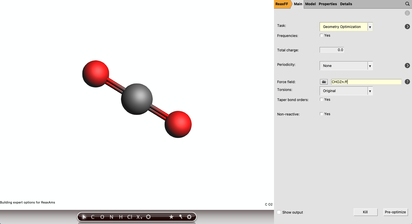
Let’s now optimize the geometry with ReaxFF.

1. Switch to ReaxFF: →

2. Select the task Geometry Optimization

3. Verify that the periodicity is set to None

4. Click the folder next to Force field and select CHOZn.ff (see Note below)

Note

If CHOZn.ff is not yet available in our database, you can download it and load it in AMS by clicking the folder icon followed by Select Any File. Then navigate to your local copy of CHOZn.ff.

Save the calculation under the name CO2_ref_ReaxFF and run the calculation. We found the total energy E_CO2 = -0.6434 Hartree = -1689.155 kJ/mol.

Host structure (IRMOF-1)

We can now import and relax the host structure.

Warning

The calculation of the full isotherm on IRMOF-1 can take several days to converge. If you would like a faster alternative, you can perform the adsorption only on a fragment of IRMOF-1 which contains 8 times less atoms. To build the fragment, we divided the supercell in 8 fragments and rotated the phenyl linker to match the periodic boundary conditions.

Download the coordinates for IRMOF-1.

1. Start a new AMSinput window

2. File → Import Coordinates (System)… and select the file IRMOF-1.xyz you just downloaded

3. Switch to the ReaxFF engine ( → )

4. Select the task Geometry Optimization

5. Verify that the periodicity is set to Bulk

6. Click the folder next to Force field and select CHOZn.ff

Note

It is also possible to relax the lattice parameter as well as to include the external pressure to the relaxation.

Save the calculation under the name IRMOF-1_ref_ReaxFF and run the calculation.

Chemical potential at constant pressure

Let’s now calculate the chemical potential to apply during the Grand-Canonical Monte Carlo simulation corresponding to some pressure range. The general formula for the chemical potential \(\mu(T,P)\) is defined as follow:

\[\begin{split}&\mu(T,P) = E_{CO2}+\Delta\mu(T,P_0)+RT\ln{\frac{P}{P_0}}\\ &\text{with }\Delta\mu(T,P_0) = H(T,P_0)-H(0,P_0)-T\times \left[S(T,P_0)-S(0,P_0)\right]\end{split}\]

The values for H and S can be extracted from reference tables such as that from the NIST website, here for CO₂. Also note that reference enthalpy and entropy values at all temperatures can be computed based on the Shomate Equation with the following coefficients (for CO₂). At 298.15 K, we found:

\[\begin{split}&\Delta\mu(298.15\text{ K},1.01\text{ bar}) = \left(0.0 - \left(-9.364\right)\right) - 298.15\times\left(0.213788 - 0.0\right) = -54.379\text{ kJ/mol} \\ &\mu(298.15\text{ K},30\text{ bar}) = -1689.155 - 54.379 + 0.008314 \times 298.15 \times \ln{\frac{3000.0}{101.325}} = -1735.136\text{ kJ/mol}\end{split}\]

The corresponding chemical potential at various pressure is summarized below:

P (bar)	5	10	15	20	25	30
µ (kJ/mol)	-1739.577	-1737.859	-1736.854	-1736.141	-1735.588	-1735.136

Note

The numbers you calculated independently might be slightly different based on the source for the enthalpy and entropy, as well as the precision and the conversion factors you used.

Grand-Canonical Monte Carlo

We can now setup the Grand-Canonical Monte Carlo simulation. We will start from the previous IRMOF-1 calculation.

1. From AMSjobs click the ReaX button left of the IRMOF-1_ref_ReaxFF calculation

2. When asked to update the coordinates say Yes

3. File → Save As… and name the calculation IRMOF-1_GCMC_ReaxFF

4. Select the task GCMC

We will freeze the host materials.

1. Model → Regions

2. Hold shift and drag the mouse to select all the atoms of the MOF

3. Click the + next to region and rename the region to host

4. Click an empty space in the molecule area to deselect atoms

5. Model → Geometry Constraints and PES Scan

6. Select one atom of the MOF

7. Click the + icon next to host (fixed position)

Let’s now setup the GCMC.

1. Model → GCMC

2. Define the Number of GCMC iterations to 100000

3. Define the Temperature to 298.15 K

4. Set Add molecules within and Add molecules not closer than to 5.0 and 1.2, respectively

And finally, we define the guest molecule.

1. Click the + icon left of Molecules

2. From Molecule select New Molecule. This will create a new empty molecule named Mol-1

3. Input the previously calculated chemical potential of -1736.141 kJ/mol (corresponding to 20 bar pressure)

Open the CO2_ref_ReaxFF and copy the optimized molecule. Click shift and drag the mouse over the molecule then key ctrl+c (or cmd+c on Mac). Then select the empty area of Mol-1 and paste the CO₂ molecule (ctrl+s / cmd+s).

We also want to set the convergence details for the geometry optimization steps in the GCMC panel.

1. Model → GCMC

2. Click the > button next to Minimization details

3. Set the Maximum number of iterations to 5000

4. In Detail → Expert AMS check Yes to Pretend converged in the Geometry Optimization section.

Note

If the maximum number of iterations is too small, high energy structures will be retained and the final load will be under-estimated. Because of the large number of degrees of freedom to optimize (especially when multiple guest molecules have been inserted), geometry optimizations might require several iterations to converge. Finding the proper number of maximum iterations requires some trial and errors. You can perform an initial GCMC with a small number of iterations (let say 1000 steps) and then look in details at the convergence of the geometry optimizations. If convergence if not well satisfied (as it was the case for IRMOF-1 with CO₂), then you can adjust the number of iterations accordingly.

Save and run the calculation. This calculation can take several days. We can post-process the results to compute and plot the acceptance ratio (the number of GCMC steps accepted over the total number of GCMC steps) and the load. From 40000 GCMC steps, we can already appreciate convergence of the load around 17 mol/kg.

Note

You can download the script to perform the GCMC analysis and plot the graph above here.

We recommend that you frequently check for convergence of the load with the script above and when you consider it has converged, you can properly stop the calculation from AMSjobs by selecting your calculation and clicking Job → Request Early Stop.

To summarize, at 20 bar and 298.15 K, we found a load of approximately 17 mol/kg. From Environ Sci Pollut Res (2014) 21:5427–5449 the experimental load is of 19 mol/kg. We show below the atomic structure of IRMOF-1 at the previously calculated load.

Note

Looking at the potential energy we can see that the GCMC is not fully converged and additional GCMC steps should be performed to obtain a well converged isotherm.

Finally, we computed the adsorption isotherm with ReaxFF based on 3 additional pressure points. We show below the adsorption isotherm computed with ReaxFF compared to experiments. The limiting loads are calculated by averaging the load over the last 40000 GCMC steps, and the error bars correspond to the standard deviation. We can conclude that CHOZn.ff reproduces well the experimental isotherm for IRMOF-1. Note that absolute isotherms for other systems might not be as accurate compared to experiment however, if the force field was well optimized (including chemistries of the host/guest well covered in the training set), we expect relative isotherms to be meaningful (in a view to optimize sorbents, for example). For production quality isotherms, we recommend to perform even more GCMC steps, and to average the load over several independent runs.