Visualization
This example demonstrates how to use the view() function, to visualize molecular and periodic systems in PLAMS.
This is further described under component View.
To follow along, either
Download
visualization.py(run as$AMSBIN/amspython visualization.py).Download
visualization.ipynb(see also: how to install Jupyterlab in AMS)
Worked Example
Visualizing Structures with PLAMS
Rendering Images
PLAMS molecules can be simply passed to the view function to render an image using AMSview. These images can then easily be displayed in a notebook.
For example, below we create a molecule of caffeine from its SMILES string, and view it.
import scm.plams as plams

caffeine = plams.from_smiles("CN1C=NC2=C1C(=O)N(C(=O)N2C)C", forcefield="uff")
plams.view(caffeine)

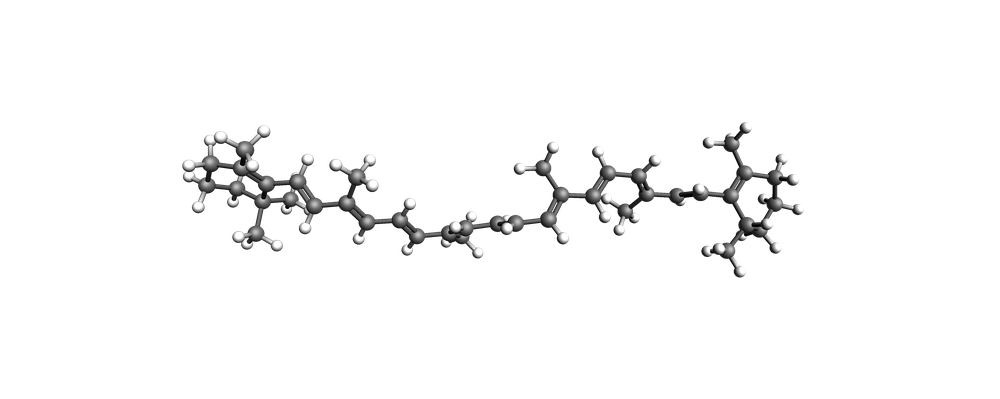
The size of the image can be controlled via the height and width arguments, which specify the size in pixels. An additional padding argument can also be used to control how much space (in Angstrom) is added or trimmed from the edges of the image.
To save the image file, the picture_path argument can be supplied which will also persist the image at the given location. Furthermore, the molecule can also be opened interactively in AMSview using the option open_window = True.
Examples of all these options are demonstrated below for beta-carotene.
beta_carotene = plams.from_smiles(
    "CC1CCC/C(C)=C1/C=C/C(C)=C/C=C/C(C)=C/C=C/C=C(C)/C=C/C=C(C)/C=C/C2=C(C)/CCCC2(C)C", forcefield="uff"
)

plams.view(
    beta_carotene,
    width=1000,
    height=400,
    padding=-7,
    picture_path="beta-carotene.png",
    open_window=True,
)
View Directions
The view method aims to make it simple to view your system in the most informative way. As such, the direction argument can be provided to change the view angle.
The direction, is composed of multiple parts and can be used to view:
along an axis
with a small_tilt, normal tilt or large_tilt
down a corner
In addition, the axis can be a:
cartesian axis - x, y, z
lattice vector - a, b, c
principal component axis - pca1, pca2, pca3
Example directions are therefore:
along_z, view along the cartesianzaxis (default value)tilt_a, view along theclattice vector with a tiltcorner_pca2, view down the corner of a principal component
Illustrations of these are provided below. Further examples can be found in the Periodic Systems section.
# Function to display three images in a row
import matplotlib.pyplot as plt


def plot_three_images(images):
    fig, axes = plt.subplots(1, 3, figsize=(16, 16))  # 1 row, 3 columns
    for i, img in enumerate(images):
        axes[i].imshow(img)
        axes[i].axis("off")
    plt.show()
images = [
    plams.view(caffeine, direction="along_x", width=400),
    plams.view(caffeine, direction="along_y", width=400),
    plams.view(caffeine, direction="along_z", width=400),
]
plot_three_images(images)

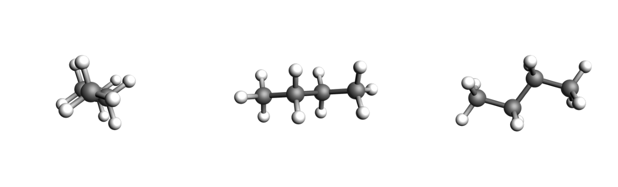
butane = plams.from_smiles("CCCC", forcefield="uff")

images = [
    plams.view(butane, direction="along_pca1", width=400),
    plams.view(butane, direction="along_pca2", width=400),
    plams.view(butane, direction="along_pca3", width=400),
]
plot_three_images(images)
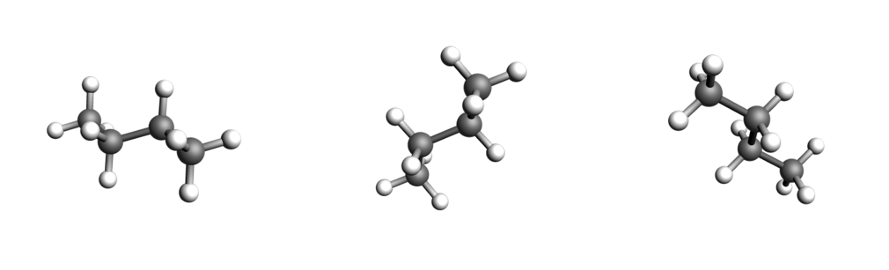
images = [
    plams.view(butane, direction="corner_pca1", width=400),
    plams.view(butane, direction="corner_pca2", width=400),
    plams.view(butane, direction="corner_pca3", width=400),
]
plot_three_images(images)
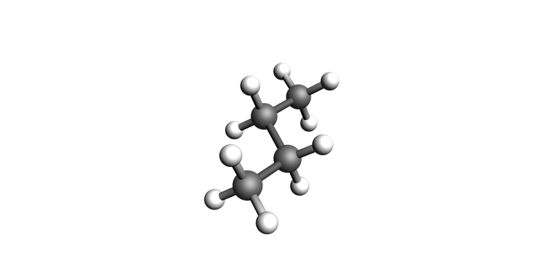
If you want finer control over the view angle, this is possible through the ViewConfig (note that more generally, all settings can be passed in via the ViewConfig, and a sub-set of the most frequently used settings can be set directly via arguments).
Here, the normal option can be provided, which specifies the normal to the view plane. The normal_basis can also be set to xyz (cartesian), abc (lattice) or pca (principal components), which defines which basis the normal vector is in.
plams.view(butane, config=plams.ViewConfig(normal=(1, 0, 1), normal_basis="pca"))
Regions and Labels
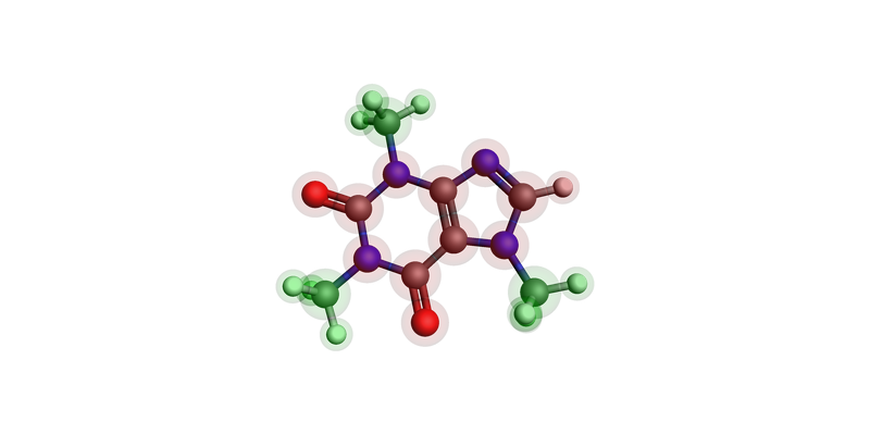
Atomic regions can be displayed by using the option show_regions=True. The regions then appear as color-coded translucent spheres on the molecule.
For example, with our caffeine molecule, we can define QM and MM regions and highlight these in the image.
# Identify methyl groups
methyl_atoms = []
for atom in caffeine.atoms:
    hydrogens = [n for n in atom.neighbors() if n.symbol == "H"]
    if atom.symbol == "C" and len(hydrogens) == 3:
        methyl_atoms.append(atom)
        methyl_atoms += hydrogens

# Set MM region as the methyl groups, QM as all other atoms
for atom in caffeine.atoms:
    if atom not in methyl_atoms:
        atom.properties.region = {"QM"}
    else:
        atom.properties.region = {"MM"}

plams.view(caffeine, show_regions=True)
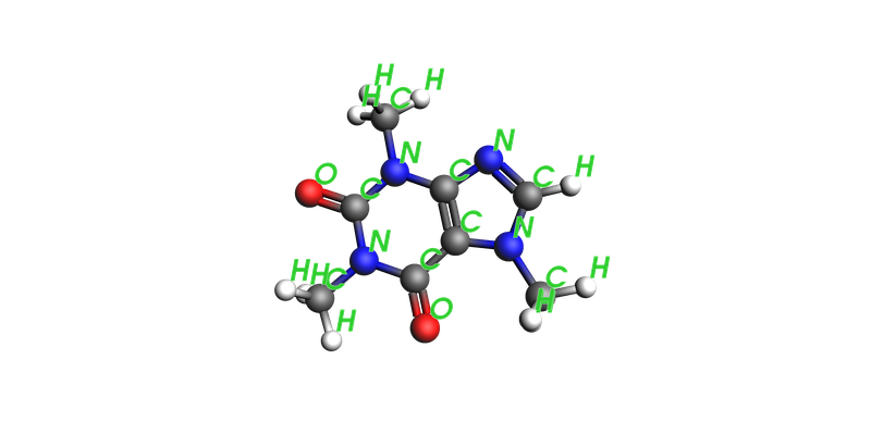
In addition, labels can also be displayed on the atoms, to indicate the elements or atom names.
These are toggled through the show_atom_labels and atom_label_type arguments. Further customization options are also available in the ViewConfig object, which can be passed to the config argument.
See the example below which also allows tuning of the atom label size and color:
plams.view(
    caffeine,
    config=plams.ViewConfig(
        show_atom_labels=True,
        atom_label_color="#32CD32",
        atom_label_size=1.7,
    ),
)
Periodic Systems
The view function works equally well for periodic systems as for molecular systems. For these systems, additional options are available for viewing the lattice and unit cell.
We set up various systems here as examples:
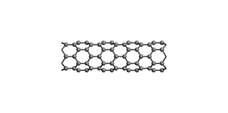
1D carbon nanotube
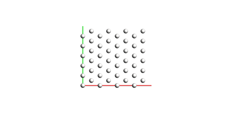
2D platinum surface
3D crystal
3D water box
First, we set up and view the carbon nanotube. By using show_unit_cell_edges=False argument we disable the default behaviour for displaying the unit cell.
import ase
import ase.build as build
import numpy as np

nanotube_atoms = build.nanotube(6, 0, length=4)
nanotube = plams.fromASE(nanotube_atoms)


# Add bonds to PLAMS molecule from neighbour list
def add_bonds(ase_atoms, mol, cutoff=1.5):
    nl_i, nl_j = ase.neighborlist.neighbor_list("ij", ase_atoms, cutoff)
    for i, j in zip(nl_i, nl_j):
        mol.add_bond(mol[i + 1], mol[j + 1])


add_bonds(nanotube_atoms, nanotube)

# Rotate from z-axis to x-axis (default in AMS)
nanotube.rotate([[0, 0, 1], [0, 1, 0], [-1, 0, 0]], lattice=True)

plams.view(nanotube, show_unit_cell_edges=False)
Next, we create the platinum surface, and use the option show_lattice_vectors=True to add the lattice vectors onto the view.
pt_surface = plams.fromASE(build.fcc111("Pt", size=(4, 4, 3), vacuum=5.0, orthogonal=True, periodic=True))
pt_surface.lattice.pop()

plams.view(pt_surface, show_unit_cell_edges=False, show_lattice_vectors=True)
Next we create a non-orthorhombic crystal structure - the wurtzite structure of zinc sulfide.
This demonstrates the further direction options that are available for periodic structures. In this case, we can also choose to view relative to the lattice vectors (a, b, c) as well as the cartesian axes (x, y, z).
For example, below we choose to view along each of the lattice vectors in turn using along_a, along_b and along_c.
Note that in this case we also set fixed_atom_size=False to scale the atoms according to their radii.
wurtzite_unit_cell = build.bulk("ZnS", crystalstructure="wurtzite", a=3.81)
wurtzite = plams.fromASE(build.make_supercell(wurtzite_unit_cell, np.diag([2, 2, 2])))

images = [
    plams.view(wurtzite, fixed_atom_size=False, show_lattice_vectors=True, direction="along_a", width=400),
    plams.view(wurtzite, fixed_atom_size=False, show_lattice_vectors=True, direction="along_b", width=400),
    plams.view(wurtzite, fixed_atom_size=False, show_lattice_vectors=True, direction="along_c", width=400),
]

plot_three_images(images)

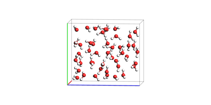
As a final example of a periodic structure, we generate an orthorhombic box of water.
Here we can also choose to view in a variety of different orientations, which emphasise the periodicity of the system. For this we set direction = tilt_x, to show the full unit cell.
In addition, we pass a ViewConfig object which exposes additional settings to fine-tune the image.
water_box = plams.packmol(
    plams.from_smiles("O"),
    density=1.0,
    box_bounds=[0.0, 0.0, 0.0, 8.0, 12.0, 14.0],
)

config = plams.ViewConfig(unit_cell_edge_thickness=0.1)
plams.view(water_box, config=config, direction="tilt_x", show_lattice_vectors=True)
Backends
By default, the view method will try and use AMSview to generate images. However, if AMSview is not available, another backend will be used. A specific backend can also be explicitly selected.
The available options are:
amsview: uses the AMSview programamsview_xvfb: for use on a headless machine (no GUI), when the Xvfb program is availablease_plot: uses ASE and matplotlib
Efforts have been made to ensure the view options when using different backends are as close as possible, and so they can simply be switched. For example, see the following images reproduced using the ASE backend:
plams.view(
    caffeine,
    width=350,
    height=350,
    show_regions=True,
    backend="ase_plot",
    show_atom_labels=True,
)

plams.view(
    water_box,
    width=350,
    height=350,
    config=config,
    direction="tilt_z",
    show_lattice_vectors=True,
    backend="ase_plot",
)

Complete Python code
#!/usr/bin/env amspython
# coding: utf-8

# ## Visualizing Structures with PLAMS

# ### Rendering Images

# PLAMS molecules can be simply passed to the `view` function to render an image using AMSview. These images can then easily be displayed in a notebook.
#
# For example, below we create a molecule of caffeine from its SMILES string, and view it.

import scm.plams as plams

caffeine = plams.from_smiles("CN1C=NC2=C1C(=O)N(C(=O)N2C)C", forcefield="uff")
plams.view(caffeine)


# The size of the image can be controlled via the `height` and `width` arguments, which specify the size in pixels. An additional `padding` argument can also be used to control how much space (in Angstrom) is added or trimmed from the edges of the image.
#
# To save the image file, the `picture_path` argument can be supplied which will also persist the image at the given location. Furthermore, the molecule can also be opened interactively in AMSview using the option `open_window = True`.
#
# Examples of all these options are demonstrated below for beta-carotene.

beta_carotene = plams.from_smiles(
    "CC1CCC/C(C)=C1/C=C/C(C)=C/C=C/C(C)=C/C=C/C=C(C)/C=C/C=C(C)/C=C/C2=C(C)/CCCC2(C)C", forcefield="uff"
)

plams.view(
    beta_carotene,
    width=1000,
    height=400,
    padding=-7,
    picture_path="beta-carotene.png",
    open_window=True,
)


# ### View Directions

# The `view` method aims to make it simple to view your system in the most informative way. As such, the `direction` argument can be provided to change the view angle.
#
# The `direction`, is composed of multiple parts and can be used to view:
#
# - __along__ an axis
# - with a __small_tilt__, normal __tilt__ or __large_tilt__
# - down a __corner__
#
# In addition, the axis can be a:
#
# - cartesian axis - __x__, __y__, __z__
# - lattice vector - __a__, __b__, __c__
# - principal component axis - __pca1__, __pca2__, __pca3__
#
# Example directions are therefore:
#
# - `along_z`, view along the cartesian `z` axis (default value)
# - `tilt_a`, view along the `c` lattice vector with a tilt
# - `corner_pca2`, view down the corner of a principal component
#
# Illustrations of these are provided below. Further examples can be found in the _Periodic Systems_ section.

# Function to display three images in a row
import matplotlib.pyplot as plt


def plot_three_images(images):
    fig, axes = plt.subplots(1, 3, figsize=(16, 16))  # 1 row, 3 columns
    for i, img in enumerate(images):
        axes[i].imshow(img)
        axes[i].axis("off")
    plt.show()


images = [
    plams.view(caffeine, direction="along_x", width=400),
    plams.view(caffeine, direction="along_y", width=400),
    plams.view(caffeine, direction="along_z", width=400),
]
plot_three_images(images)


butane = plams.from_smiles("CCCC", forcefield="uff")

images = [
    plams.view(butane, direction="along_pca1", width=400),
    plams.view(butane, direction="along_pca2", width=400),
    plams.view(butane, direction="along_pca3", width=400),
]
plot_three_images(images)


images = [
    plams.view(butane, direction="corner_pca1", width=400),
    plams.view(butane, direction="corner_pca2", width=400),
    plams.view(butane, direction="corner_pca3", width=400),
]
plot_three_images(images)


# If you want finer control over the view angle, this is possible through the `ViewConfig` (note that more generally, all settings can be passed in via the `ViewConfig`, and a sub-set of the most frequently used settings can be set directly via arguments).
#
# Here, the `normal` option can be provided, which specifies the normal to the view plane. The `normal_basis` can also be set to `xyz` (cartesian), `abc` (lattice) or `pca` (principal components), which defines which basis the normal vector is in.

plams.view(butane, config=plams.ViewConfig(normal=(1, 0, 1), normal_basis="pca"))


# ### Regions and Labels

# Atomic regions can be displayed by using the option `show_regions=True`. The regions then appear as color-coded translucent spheres on the molecule.
#
# For example, with our caffeine molecule, we can define QM and MM regions and highlight these in the image.

# Identify methyl groups
methyl_atoms = []
for atom in caffeine.atoms:
    hydrogens = [n for n in atom.neighbors() if n.symbol == "H"]
    if atom.symbol == "C" and len(hydrogens) == 3:
        methyl_atoms.append(atom)
        methyl_atoms += hydrogens

# Set MM region as the methyl groups, QM as all other atoms
for atom in caffeine.atoms:
    if atom not in methyl_atoms:
        atom.properties.region = {"QM"}
    else:
        atom.properties.region = {"MM"}

plams.view(caffeine, show_regions=True)


# In addition, labels can also be displayed on the atoms, to indicate the elements or atom names.
#
# These are toggled through the `show_atom_labels` and `atom_label_type` arguments. Further customization options are also available in the `ViewConfig` object, which can be passed to the `config` argument.
#
# See the example below which also allows tuning of the atom label size and color:

plams.view(
    caffeine,
    config=plams.ViewConfig(
        show_atom_labels=True,
        atom_label_color="#32CD32",
        atom_label_size=1.7,
    ),
)


# ## Periodic Systems

# The `view` function works equally well for periodic systems as for molecular systems. For these systems, additional options are available for viewing the lattice and unit cell.
#
# We set up various systems here as examples:
#
# - 1D carbon nanotube
# - 2D platinum surface
# - 3D crystal
# - 3D water box

# First, we set up and view the carbon nanotube. By using `show_unit_cell_edges=False` argument we disable the default behaviour for displaying the unit cell.

import ase
import ase.build as build
import numpy as np

nanotube_atoms = build.nanotube(6, 0, length=4)
nanotube = plams.fromASE(nanotube_atoms)


# Add bonds to PLAMS molecule from neighbour list
def add_bonds(ase_atoms, mol, cutoff=1.5):
    nl_i, nl_j = ase.neighborlist.neighbor_list("ij", ase_atoms, cutoff)
    for i, j in zip(nl_i, nl_j):
        mol.add_bond(mol[i + 1], mol[j + 1])


add_bonds(nanotube_atoms, nanotube)

# Rotate from z-axis to x-axis (default in AMS)
nanotube.rotate([[0, 0, 1], [0, 1, 0], [-1, 0, 0]], lattice=True)

plams.view(nanotube, show_unit_cell_edges=False)


# Next, we create the platinum surface, and use the option `show_lattice_vectors=True` to add the lattice vectors onto the view.

pt_surface = plams.fromASE(build.fcc111("Pt", size=(4, 4, 3), vacuum=5.0, orthogonal=True, periodic=True))
pt_surface.lattice.pop()

plams.view(pt_surface, show_unit_cell_edges=False, show_lattice_vectors=True)


# Next we create a non-orthorhombic crystal structure - the wurtzite structure of zinc sulfide.
#
# This demonstrates the further `direction` options that are available for periodic structures. In this case, we can also choose to view relative to the lattice vectors (`a`, `b`, `c`) as well as the cartesian axes (`x`, `y`, `z`).
#
# For example, below we choose to view along each of the lattice vectors in turn using `along_a`, `along_b` and `along_c`.
#
# Note that in this case we also set `fixed_atom_size=False` to scale the atoms according to their radii.

wurtzite_unit_cell = build.bulk("ZnS", crystalstructure="wurtzite", a=3.81)
wurtzite = plams.fromASE(build.make_supercell(wurtzite_unit_cell, np.diag([2, 2, 2])))

images = [
    plams.view(wurtzite, fixed_atom_size=False, show_lattice_vectors=True, direction="along_a", width=400),
    plams.view(wurtzite, fixed_atom_size=False, show_lattice_vectors=True, direction="along_b", width=400),
    plams.view(wurtzite, fixed_atom_size=False, show_lattice_vectors=True, direction="along_c", width=400),
]

plot_three_images(images)


# As a final example of a periodic structure, we generate an orthorhombic box of water.
#
# Here we can also choose to view in a variety of different orientations, which emphasise the periodicity of the system. For this we set `direction = tilt_x`, to show the full unit cell.
#
# In addition, we pass a `ViewConfig` object which exposes additional settings to fine-tune the image.

water_box = plams.packmol(
    plams.from_smiles("O"),
    density=1.0,
    box_bounds=[0.0, 0.0, 0.0, 8.0, 12.0, 14.0],
)

config = plams.ViewConfig(unit_cell_edge_thickness=0.1)
plams.view(water_box, config=config, direction="tilt_x", show_lattice_vectors=True)


# ### Backends

# By default, the `view` method will try and use AMSview to generate images. However, if AMSview is not available, another backend will be used. A specific backend can also be explicitly selected.
#
# The available options are:
#
# - `amsview`: uses the AMSview program
# - `amsview_xvfb`: for use on a headless machine (no GUI), when the [Xvfb](https://www.x.org/archive/X11R7.7/doc/man/man1/Xvfb.1.xhtml) program is available
# - `ase_plot`: uses ASE and matplotlib
#
# Efforts have been made to ensure the view options when using different backends are as close as possible, and so they can simply be switched. For example, see the following images reproduced using the ASE backend:

plams.view(
    caffeine,
    width=350,
    height=350,
    show_regions=True,
    backend="ase_plot",
    show_atom_labels=True,
)


plams.view(
    water_box,
    width=350,
    height=350,
    config=config,
    direction="tilt_z",
    show_lattice_vectors=True,
    backend="ase_plot",
)