Examples
These examples show how to run Quantum ESPRESSO through the AMS driver.
All examples can be run from the command-line and most of them are also available in
$AMSHOME/examples/QEMost of the examples can also be copy-pasted or opened directly in the AMSinput GUI
Important
These examples do not necessarily contain scientifically good settings!
Typically you should increase the energy cutoff and k-point sampling for scientifically good results.
See also
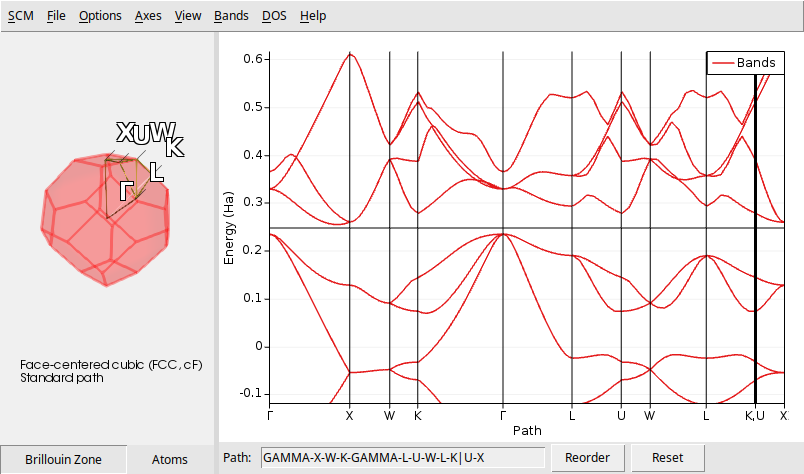
Single-Point Calculation + Band Structure
Input File (run from command-line or the AMSinput GUI)
#!/bin/sh

export SCM_DISABLE_MPI=1  # must be set when using the Quantum ESPRESSO engine, see documentation

"$AMSBIN/ams" --delete-old-results << EOF
Task SinglePoint

System
    Atoms
        Si      -0.67520366      -0.67520366      -0.67520366
        Si       0.67520366       0.67520366       0.67520366
    End
    Lattice
        0.00000000       2.70081465       2.70081465
        2.70081465       0.00000000       2.70081465
        2.70081465       2.70081465       0.00000000
    End
End

Engine QuantumEspresso
    System
       ecutwfc 50
       ecutrho 400
       occupations smearing
       degauss 0.001
    End
    K_Points automatic
        5 5 5 0 0 0
    End
    Pseudopotentials
        Family pslibrary-US
        Functional PBE
    End
    Properties
        BandStructure Yes
    End
EndEngine
EOF
Single-point calculation for bulk silicon using a regular Monkhorst-Pack k-point grid.
The electronic band structure is calculated along high-symmetry lines in the Brillouin zone.
You can view the resulting band structure with the program
$AMSBIN/amsbands.
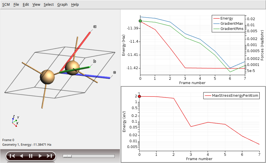
Lattice Optimization of Silicon
Input File (run from command-line or the AMSinput GUI)
#!/bin/sh

export SCM_DISABLE_MPI=1  # required for Quantum ESPRESSO - see documentation

#============================================================================
# Example showing how to run a lattice optimization with Quantum ESPRESSO.
#
# This example is also available as a tutorial using the
# graphical user interface
#
# Important: always use carefully converged k-points and energy cutoffs
# for lattice optimizations!
#
# You may want to symmetrize the optimized structure using the "star"
# button in AMSinput.
#============================================================================

"$AMSBIN/ams" --delete-old-results <<EOF
Task GeometryOptimization

GeometryOptimization
    OptimizeLattice Yes
End

System
    Atoms
        Si      -0.67875000      -0.67875000      -0.67875000
        Si       0.67875000       0.67875000       0.67875000
    End
    Lattice
        0.0 3.0 3.0
        3.0 0.0 3.0
        3.0 3.0 0.0
    End
End

Engine QuantumEspresso
    K_Points automatic
        10 10 10 0 0 0
    End
    Pseudopotentials
        Family SSSP-Efficiency
        Functional PBE
    End
    System
        ecutwfc 40.0
        ecutrho 320.0
        occupations Fixed
    End
EndEngine
EOF
Full structural optimization of bulk silicon
Both the atomic positions and lattice parameters are relaxed
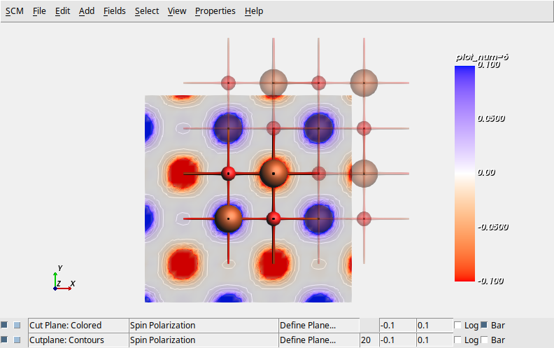
DFT+U (Hubbard U) Calculation for Anti-ferromagnetic FeO
Input File (run from command-line or the AMSinput GUI)
#!/bin/sh

# Run AMS driver without MPI, so that QE can be MPI parallel.
export SCM_DISABLE_MPI=1

"$AMSBIN/ams" --delete-old-results << EOF

Task SinglePoint

System
    Atoms
        Fe  0.0    0.0    0.0   QE.Label=Fe1
        Fe  2.165  2.165  0.0   QE.Label=Fe2
        O   0.0    2.165  0.0
        O   2.165  0.0    0.0
    End
    Lattice
        4.33   0.0   0.0
        0.0    4.33  0.0
        2.165  0.0   2.165
    End
End

Engine QuantumEspresso
   System
       ecutwfc 40.0
       ecutrho 160.0
       occupations smearing
       smearing mv
       degauss 0.02
       nspin 2
       starting_magnetization label=Fe1 value=0.5
       starting_magnetization label=Fe2 value=-0.5
   End
   Pseudopotentials
      Family pslibrary-PAW
      Functional PBEsol
   End
   K_Points automatic
      5 5 5 0 0 0
   End
   Hubbard ortho-atomic
      U Fe1-3d 4.6
      U Fe2-3d 4.6
   End
EndEngine

EOF
DFT+U calculation for antiferromagnetic FeO
The
QE.Label=keyword is employed to define distinct Fe speciesThe
starting_magnetizationkeyword refers to the labels to give different initial spin magnetizations, leading to an anti-ferromagnetic solution.Hubbard U is specified in the new Quantum ESPRESSO 7.1 format
Pseudopotential Selection
Command-line runscript
#!/bin/sh

export SCM_DISABLE_MPI=1  # required for engine Quantum ESPRESSO, see documentation


# =======================================================================================
# Example illustrating various ways of selecting Pseudopotentials with the QE engine.
# =======================================================================================
#
# All jobs run into this example should give the exact same result,
# as they are using the same PPs.
# All that differs is the way that the PPs were selected.


# Make a folder with "custom" PP files to test with:
#
# We will use the SG15 pseudopotentials directory that comes
# with the AMS QE package as an example.
# You could use any other directory with .upf files ...
PPDIR="$("$AMSBIN/amspackages" loc qe)/upf_files/GGA/PBE/SR/SG15-1.2/UPFs"

# Make a custom directory containing files named element.upf:
mkdir -p my_pp_directory
cp "$PPDIR"/C_ONCV_PBE-1.2.upf my_pp_directory/C.upf  # rename to element.upf
cp "$PPDIR"/H_ONCV_PBE-1.2.upf my_pp_directory/H.upf  # rename to element.upf

# If using special QE labels, the file name should be label.upf:
cp "$PPDIR"/H_ONCV_PBE-1.2.upf my_pp_directory/H1.upf

# Get an absolute path to the directory the jobs starts in:
if test "$OS" = "Windows_NT"; then
    # Absolute paths should be Windows style (with drive letters like C:)
    STARTDIR=$(pwd -W)
else
    STARTDIR=$(pwd)
fi


# Make a system to test with:
echo "
    System
        Atoms
            C 0.9685 1.9663  0.0000
            H 1.6614 2.2162  0.7898
            H 0.0162 1.6927  0.4297
            H 0.8388 2.8201 -0.6485
            H 1.3576 1.1363 -0.5710 QE.Label=H1
        End
        Lattice
            5.0 0.0 0.0
            0.0 5.0 0.0
            0.0 0.0 5.0
        End
    End
" > system.in


# Option 1: Pseudopotentials%Family
# ---------------------------------
#
# The easiest way is to just use the Pseudopotentials%Family key and
# let the engine figure out which PPs to use.

AMS_JOBNAME=1_family "$AMSBIN/ams" << EOF
    Task SinglePoint
    @include system.in

    Engine QuantumEspresso
        Pseudopotentials
            Family SG15
            Functional PBE
        End
        K_points Gamma
        End
    EndEngine
EOF


# Option 2: Pseudopotentials%Directory
# ------------------------------------
#
# Specifies a path to a directory with PP files named element.upf or label.upf.
# The path to the directory can be absolute or relative.

AMS_JOBNAME=2a_directory_relpath "$AMSBIN/ams" << EOF
    Task SinglePoint
    @include system.in

    Engine QuantumEspresso
        Pseudopotentials
            Directory my_pp_directory
        End
        K_points Gamma
        End
    EndEngine
EOF

AMS_JOBNAME=2b_directory_abspath "$AMSBIN/ams" << EOF
    Task SinglePoint

    System
        Atoms
            C 0.9685 1.9663  0.0000 QE.Label=C1  # no PP file for C1 in folder, fallback to C
            H 1.6614 2.2162  0.7898
            H 0.0162 1.6927  0.4297
            H 0.8388 2.8201 -0.6485
            H 1.3576 1.1363 -0.5710 QE.Label=H1
        End
        Lattice
            5.0 0.0 0.0
            0.0 5.0 0.0
            0.0 0.0 5.0
        End
    End

    Engine QuantumEspresso
        Pseudopotentials
            Directory $STARTDIR/my_pp_directory
        End
        K_points Gamma
        End
    EndEngine
EOF


# Option 3: Pseudopotentials%Files
# ------------------------------------
#
# Individually specify paths to files for each element or label.

# By default relative paths are relative to the root of the
# PP library installed via AMSpackages.

AMS_JOBNAME=3a_files_relpath "$AMSBIN/ams" << EOF
    Task SinglePoint
    @include system.in

    Engine QuantumEspresso
        Pseudopotentials
            Files Label=C  Path=GGA/PBE/SR/SG15-1.2/UPFs/C_ONCV_PBE-1.2.upf
            Files Label=H  Path=GGA/PBE/SR/SG15-1.2/UPFs/H_ONCV_PBE-1.2.upf
            Files Label=H1 Path=GGA/PBE/SR/SG15-1.2/UPFs/H_ONCV_PBE-1.2.upf
        End
        K_points Gamma
        End
    EndEngine
EOF

# Paths relative to the starting directory of AMS should be prefixed with "./".

AMS_JOBNAME=3b_files_exrelpath "$AMSBIN/ams" << EOF
    Task SinglePoint
    @include system.in

    Engine QuantumEspresso
        Pseudopotentials
            Files Label=C  Path=./my_pp_directory/C.upf
            Files Label=H  Path=./my_pp_directory/H.upf
            Files Label=H1 Path=./my_pp_directory/H1.upf
        End
        K_points Gamma
        End
    EndEngine
EOF

# Absolute paths are also supported.

AMS_JOBNAME=3c_files_abspath "$AMSBIN/ams" << EOF
    Task SinglePoint
    @include system.in

    Engine QuantumEspresso
        Pseudopotentials
            Files Label=C  Path="$STARTDIR/my_pp_directory/C.upf"
            Files Label=H  Path="$STARTDIR/my_pp_directory/H.upf"
            Files Label=H1 Path="$STARTDIR/my_pp_directory/H1.upf"
        End
        K_points Gamma
        End
    EndEngine
EOF

# Combinations between absolute, relative and explicit relative paths also work.

AMS_JOBNAME=3d_files_mixed "$AMSBIN/ams" << EOF
    Task SinglePoint
    @include system.in

    Engine QuantumEspresso
        Pseudopotentials
            Files Label=C  Path=GGA/PBE/SR/SG15-1.2/UPFs/C_ONCV_PBE-1.2.upf
            Files Label=H  Path=./my_pp_directory/H.upf
            Files Label=H1 Path="$STARTDIR/my_pp_directory/H1.upf"
        End
        K_points Gamma
        End
    EndEngine
EOF
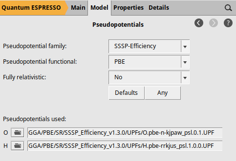
This example illustrates various methods for selecting pseudopotentials. It covers:
Pseudopotentials%Family: Predefined sets for simple selection.Pseudopotentials%Directory: Directory containing filesH.upf,He.upf, etc.Pseudopotentials%Files: Specify each individual pseudopotential file (similar to standalone Quantum ESPRESSO).
All these options are also accessible from the AMSinput GUI.
Slab With Dipole Correction, Work Function
Input File (run from command-line or the AMSinput GUI)
#!/bin/sh

export SCM_DISABLE_MPI=1
export AMS_JOBNAME=DipoleCorrection_WorkFunction

#============================================================================
# Example showing how to apply a dipole correction for a slab system.
# This gives two separate vacuum levels on the different sides of the slab.
# The respective work functions are calculated as differences
# between the vacuum levels and the Fermi energy.
#
# This example uses internally the pp.x and average.x utilities from Quantum
# ESPRESSO to get the plane-averaged electrostatic potential.
#
# For details about the input to pp.x, and average.x, see:
#  - https://www.quantum-espresso.org/Doc/INPUT_PP.html
#  - https://gitlab.com/QEF/q-e/-/blob/qe-7.1/PP/src/average.f90
#
# This example is based on the work function tutorial for BAND and the
# work function example in Quantum ESPRESSO (PP/examples/WorkFct_example).
#
# Better-converged numbers can be obtained by increasing the k-space
# sampling and energy cutoff.
#============================================================================

"$AMSBIN/ams" --delete-old-results <<EOF
Task SinglePoint

System
    Atoms
        Al 1.4319 1.4319 8.925
        Al 0.0000 0.0000 10.95
        Al 1.4319 1.4319 12.975
        Al 0.0000 0.0000 15
        F 0.0000 0.0000 18.27
        Li 1.4319 1.4319 18.27
        F 1.4319 1.4319 20.295
        Li 0.0000 0.0000 20.295
    End
    Lattice
       2.86378246       0.00000000       0.00000000
       0.00000000       2.86378246       0.00000000
       0.0 0.0 30.0
    End
End

Engine QuantumEspresso
    K_Points automatic
        2 2 1 1 1 1
    End
    Pseudopotentials
        Family GBRV
        Functional PBE
    End
    System
        ecutwfc 40.0
        occupations smearing
        smearing gaussian
        degauss 0.02
        edir 3
        emaxpos 0.90
        eopreg 0.10
    End
    Electrons
        conv_thr 1.0e-10
    End
    Control
        tefield Yes
        dipfield Yes
    End
    Properties
        WorkFunction Yes
    End
EndEngine
EOF

$AMSBIN/amspython -c '
import scm.plams
import matplotlib.pyplot as plt

job = scm.plams.AMSJob.load_external("'$AMS_JOBNAME'.results/ams.rkf")

wf_results = job.results.get_work_function_results( "eV", "Angstrom" )
ax = scm.plams.plot_work_function(*wf_results)

ax.set_title("Electrostatic Potential Profile", fontsize=14)
ax.set_xlabel("Shifted coordinate (angstrom)", fontsize=13)
ax.set_ylabel("Electrostatic potential (eV)", fontsize=13)

plt.savefig("work_function.png")
'
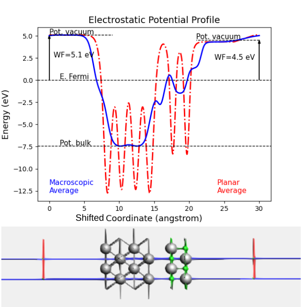
Recommended: Place the system in the middle of the unit cell to calculate the work function.
Apply a dipole correction to account for the dipole moment across the vacuum between periodic images
This gives two separate vacuum levels on the different sides of the slab
The work functions are calculated as the difference between the vacuum level and the Fermi energy.
Numerical Calculation of Phonons
Input File (run from command-line or the AMSinput GUI)
#!/bin/sh

export SCM_DISABLE_MPI=1

AMS_JOBNAME=DiamondNumericalPhonons_Curtarolo "$AMSBIN/ams" --delete-old-results << EOF
Task SinglePoint

System
    Atoms
        C    -0.44625000    -0.44625000    -0.44625000
        C     0.44625000     0.44625000     0.44625000
    End
    Lattice
         0.00000000     1.78500000     1.78500000
         1.78500000     0.00000000     1.78500000
         1.78500000     1.78500000     0.00000000
    End
End

Properties
    Phonons Yes
End

Phonons
    Method Numerical
End

NumericalPhonons
    SuperCell
        2 0 0
        0 2 0
        0 0 2
    End
    AutomaticBZPath Yes
End

Engine QuantumEspresso
    K_Points automatic
        3 3 3 0 0 0
    End
EndEngine

EOF

# This section uses PLAMS to plot the phonons bands in a Python environment
AMS_JOBNAME=DiamondNumericalPhonons_Curtarolo $AMSBIN/amspython -c '
import os
import scm.plams
import matplotlib.pyplot as plt

results_file = os.environ["AMS_JOBNAME"]+".results/ams.rkf"
job = scm.plams.AMSJob.load_external(results_file)

phonons_data = job.results.get_phonons_band_structure(unit="cm^-1")
ax = scm.plams.plot_phonons_band_structure(*phonons_data)
ax.set_ylabel("$E$ (cm$^{-1}$)")
ax.set_xlabel("Path")
ax.set_title("Diamond Phonons")
plt.savefig("phonons.png")

properties_data = job.results.get_phonons_thermodynamic_properties( properties_unit=["kJ/mol", "J/K/mol"] )
ax = scm.plams.plot_phonons_thermodynamic_properties(*properties_data)
ax.set_ylabel("Thermodynamic Properties")
ax.set_xlabel("Temperature (K)")
plt.savefig("thermodynamics.png")
'
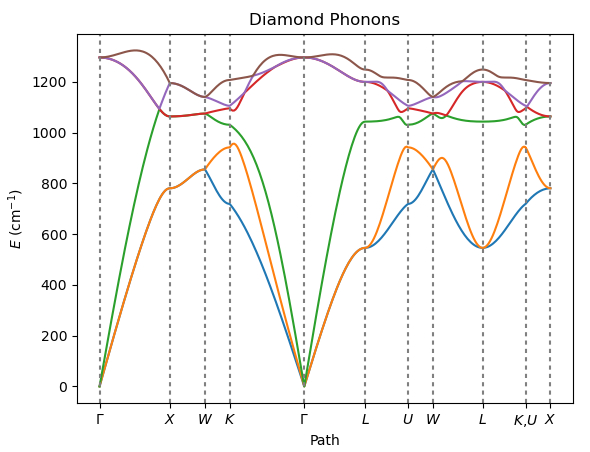
Calculate phonon dispersion curves of diamond using numerical differentiation.
The dynamical matrix is constructed within the supercell approximation by computing forces resulting from finite atomic displacements.
Visualize the results with the AMSbands GUI or the Python PLAMS library.
Analytical Calculation of Phonons Using DFPT
Input File (run from command-line or the AMSinput GUI)
#!/bin/sh

export SCM_DISABLE_MPI=1

AMS_JOBNAME=DiamondPhonons_Curtarolo "$AMSBIN/ams" --delete-old-results << EOF
Task SinglePoint

System
    Atoms
        C    -0.44625000    -0.44625000    -0.44625000
        C     0.44625000     0.44625000     0.44625000
    End
    Lattice
         0.00000000     1.78500000     1.78500000
         1.78500000     0.00000000     1.78500000
         1.78500000     1.78500000     0.00000000
    End
End

Properties
    Phonons Yes
End

Engine QuantumEspresso
    K_Points automatic
        3 3 3 0 0 0
    End
    Phonons
        asr crystal
        Q_Points automatic
           4 4 4 0 0 0
        End
    End
EndEngine

EOF

# This section uses PLAMS to plot the phonons bands in a Python environment
AMS_JOBNAME=DiamondPhonons_Curtarolo $AMSBIN/amspython -c '
import os
import scm.plams
import matplotlib.pyplot as plt

results_file = os.environ["AMS_JOBNAME"]+".results/ams.rkf"
job = scm.plams.AMSJob.load_external(results_file)

phonons_data = job.results.get_phonons_band_structure(unit="cm^-1")
ax = scm.plams.plot_phonons_band_structure(*phonons_data)
ax.set_ylabel("$E$ (cm$^{-1}$)")
ax.set_xlabel("Path")
ax.set_title("Diamond Phonons")
plt.savefig("phonons.png")

properties_data = job.results.get_phonons_thermodynamic_properties( properties_unit=["kJ/mol", "J/K/mol"] )
ax = scm.plams.plot_phonons_thermodynamic_properties(*properties_data)
ax.set_ylabel("Thermodynamic Properties")
ax.set_xlabel("Temperature (K)")
plt.savefig("thermodynamics.png")
'
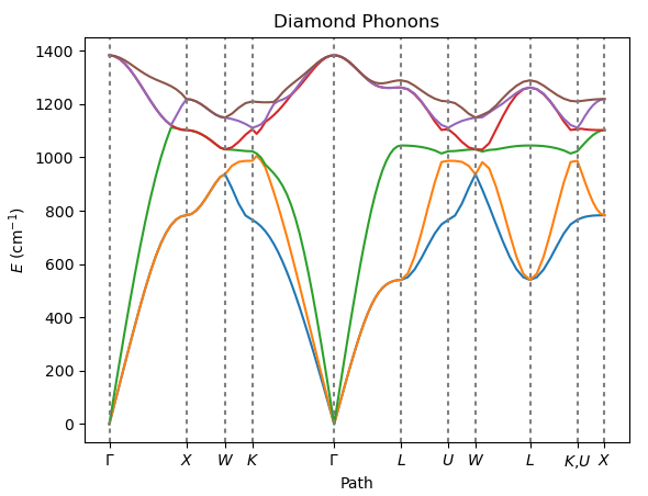
Calculate phonon dispersion curves of diamond using Density Functional Perturbation Theory (DFPT) as implemented in Quantum ESPRESSO.
DFPT allows for the analytical computation of the dynamical matrix.
Visualize the results with the AMSbands GUI or the Python PLAMS library.
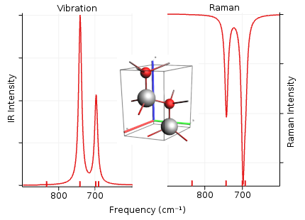
IR/Raman Spectra
Input File (run from command-line or the AMSinput GUI)
#!/bin/sh

export SCM_DISABLE_MPI=1
export AMS_JOBNAME=BeO

"$AMSBIN/ams" --delete-old-results << EOF

Task GeometryOptimization

Properties
  NormalModes Yes
  Raman Yes
End

System
  Atoms
             Be       0.0000000000       1.5555413800       0.0007009000
             Be       1.3471383600       0.7777706900       2.1887103500
              O       0.0000000000       1.5555413800       1.6512462200
              O       1.3471383600       0.7777706900       3.8392556700
  End
  Lattice
         2.6942767100     0.0000000000     0.0000000000
        -1.3471383600     2.3333120800     0.0000000000
         0.0000000000     0.0000000000     4.3760188900
  End
End

Engine QuantumEspresso
  System
    ecutwfc 25.0
  End
  K_Points automatic
     4 4 4 0 0 0
  End
  Pseudopotentials
    Files Label=Be Path=QE/Be.pz-mt_fhi.UPF
    Files Label=O Path=QE/O.pz-mt_fhi.UPF
  End
EndEngine

EOF
Calculate the infrared and Raman spectra of BeO using DFPT
Use norm-conserving pseudopotentials
Raman only available for LDA
Visualize the calculated IR and Raman spectra, and also the corresponding vibrational modes with the program
$AMSBIN/amsspectra
PESScan: volume scan
Input File (run from command-line or the AMSinput GUI)
#!/bin/sh

export SCM_DISABLE_MPI=1

"$AMSBIN/ams" --delete-old-results <<EOF

Task PESScan
System
    Atoms
        Mg 0.000 0.000 0.000
         O 2.105 2.105 2.105
    End
    Lattice
        0.000 2.105 2.105
        2.105 0.000 2.105
        2.105 2.105 0.000
    End
End
PESScan
    CalcPropertiesAtPESPoints Yes
    ScanCoordinate
        nPoints 5
        CellVolumeScalingRange 0.9 1.2
    End
End

Engine QuantumEspresso
    K_Points automatic
        2 2 2 0 0 0
    End
    Properties
       DOS Yes
       BandStructure Yes
    End
    DOS
        K_Points automatic
            10 10 10 0 0 0
        End
    End
    BandStructure
        K_Points ams_kpath
        End
    End
EndEngine

EOF
Use the
PESScantask in combination with the Quantum ESPRESSO engine. It performs a series of geometry optimization calculations while systematically varying the cell volume of MgO.The density of states (DOS) and band structure are calculated for each volume.
You can analyze the results with the program
$AMSBIN/amsmovie.
Replay
Command-line runscript
#!/bin/sh

export SCM_DISABLE_MPI=1

AMS_JOBNAME=PESScan "$AMSBIN/ams" --delete-old-results <<EOF

Task PESScan

System
    Atoms
        Mg 0.000 0.000 0.000
         O 2.105 2.105 2.105
    End
    Lattice
        0.000 2.105 2.105
        2.105 0.000 2.105
        2.105 2.105 0.000
    End
End

PESScan
    ScanCoordinate
        nPoints 3
        CellVolumeScalingRange 0.9 1.2
    End
End

Engine QuantumEspresso
    K_Points automatic
        2 2 2 0 0 0
    End
EndEngine

EOF

AMS_JOBNAME=Replay "$AMSBIN/ams" --delete-old-results << EOF

Task Replay

Replay
    File PESScan.results/ams.rkf
End

Properties
    Gradients Yes
    StressTensor Yes
End

Engine QuantumEspresso
    K_Points automatic
        5 5 5 0 0 0
    End
EndEngine

EOF
This example demonstrates a two-step approach for efficient property calculations. Initially, a PESScan task is performed with a low-precision setup (e.g., coarse k-point grid) to quickly generate a series of structures, using a cell volume scaling for MgO as a prototype system. Then, the Replay task is used to evaluate properties like gradients and stress tensors at a higher precision (e.g., finer k-point grid) for the selected structures.
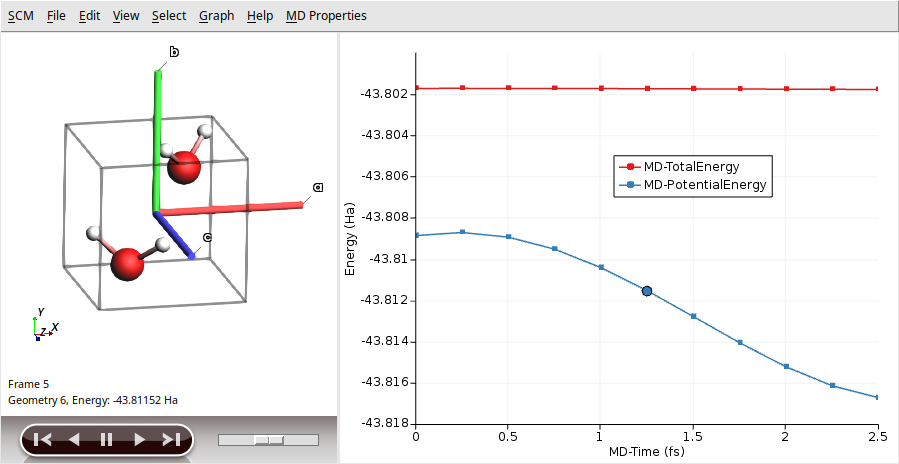
Born-Oppenheimer Molecular Dynamics
Input File (run from command-line or the AMSinput GUI)
#!/bin/sh

export SCM_DISABLE_MPI=1

AMS_JOBNAME=MolecularDynamics "$AMSBIN/ams" --delete-old-results << EOF

Task MolecularDynamics
RNGSeed 10

MolecularDynamics
    NSteps 10
    Trajectory
        SamplingFreq 1
        EngineResultsFreq 0
    End
    Checkpoint
        Frequency 1
    End
    InitialVelocities
        Temperature 300
    End
End

System
    Atoms
        O  0.77656125  0.70226469 -0.77898886
        H  0.18695701  1.27832345 -0.18188342
        H  1.36427986  1.27137397 -1.38443744
        O -0.77660318 -0.83048394  0.77894720
        H -0.18661066 -0.26385475  1.38473471
        H -1.36396069 -0.25091023  0.18224739
    End
    Lattice
         3.10979012 0.00175445 -0.000372438
        -0.00721068 3.06655157 -0.007924867
        -3.8697e-05 0.00424969  3.111852930
    End
End

Engine QuantumEspresso
EndEngine

EOF
Born-Oppenheimer Molecular Dynamics (BOMD) simulation with the AMS Driver
Analyze the resulting trajectory with the program
$AMSBIN/amsmovie
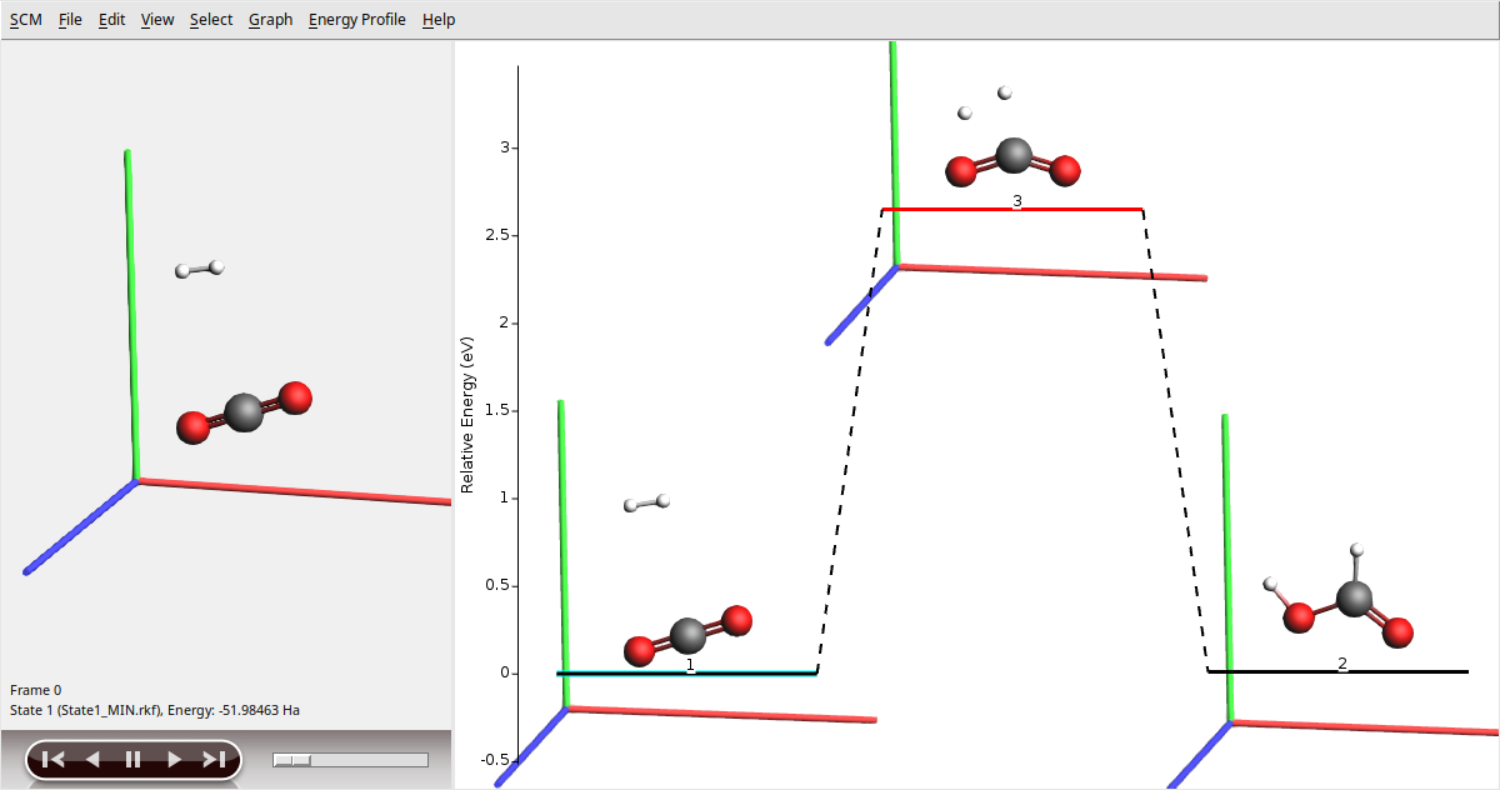
PES Exploration
Input File (run from command-line or the AMSinput GUI)
#!/bin/sh

export SCM_DISABLE_MPI=1

"$AMSBIN/ams" --delete-old-results << EOF

Task PESExploration
PESExploration
    Job SaddleSearch
    RandomSeed 10
    Optimizer
        ConvergedForce 0.05
    End
    SaddleSearch
        DisplaceMagnitude 0.01
        RelaxFromSaddlePoint Yes
    End
End
System
    Atoms
        O       3.63620880       3.57049155       4.48487828
        C       4.48799778       4.50659100       4.51176734
        O       5.64352871       4.78595471       4.54849633
        H       3.09645968       4.80015429       4.45130367
        H       3.65975624       5.66218780       4.46883580
    End
    Lattice
        9.0 0.0 0.0
        0.0 9.0 0.0
        0.0 0.0 9.0
    End
End

Engine QuantumEspresso
    System
        ecutwfc 30.0
        ecutrho 120.0
        assume_isolated Martyna-Tuckerman
    End
    K_Points automatic
        1 1 1 0 0 0
    End
    NormalModes
        asr crystal
    End
EndEngine

EOF
This example demonstrates the use of the Quantum ESPRESSO engine in combination with the PESExploration task. The initial structure is a guess to the transition state of the reaction \(H_2+CO_2 \longrightarrow HOCHO\). Here, AMS locates the actual transition state and the corresponding reactants and products in an automated fashion.