PES point properties¶

No matter what application the AMS driver is used for, in one way or another it always explores the potential energy surface (PES) of the system. One can furthermore ask AMS to calculate additional properties of the PES in the points that are visited. These are mostly (but not exclusively) derivatives of the energy, e.g. we can ask AMS to calculate the gradients or the Hessian in the visited points. In general all these PES point properties are requested through the Properties block in the AMS input:

Properties
   Gradients [True | False]
   StressTensor [True | False]
   Hessian [True | False]
   SelectedAtomsForHessian integer_list
   NormalModes [True | False]
   PESPointCharacter [True | False]
   ElasticTensor [True | False]
   Phonons [True | False]
   DipoleMoment [True | False]
   BondOrders [True | False]
End

This page in the AMS manual describes all the supported properties.

Note that because these properties are tied to a particular point on the potential energy surface, they are found on the engine output files. Note also that the properties are not always calculated in every PES point that the AMS driver visits during a calculation. By default they are only calculated in special PES points, where the definition of special depends on the task AMS is performing: For a geometry optimization properties would for example only be calculated at the final, converged geometry. This behavior can often be modified by keywords special to the particular running task.

Nuclear gradients and stress tensor¶

The first derivative with respect to the nuclear coordinates can be requested as follows:

Properties
   Gradients [True | False]
End

Properties

Gradients

Type:	Bool
Default value:	False
GUI name:	Nuclear gradients
Description:	Calculate the nuclear gradients.

Note that these are gradients, not forces, the difference being the sign. The gradients are printed in the output and written to the engine result file belonging to the particular point on the PES in the AMSResults%Gradients variable as a \(3 \times n_\mathrm{atoms}\) array in atomic units (Hartree/Bohr).

For periodic systems (chains, slabs, bulk) one can also request the clamped-ion stress tensor (note: the clamped-ion stress is only part of the true stress tensor):

Properties
   StressTensor [True | False]
End

Properties

StressTensor

Type:	Bool
Default value:	False
GUI name:	Stress tensor
Description:	Calculate the stress tensor.

The clamped-ion stress tensor \(\sigma_\alpha\) (Voigt notation) is computed via numerical differentiation of the energy \(E\) WRT a strain deformations \(\epsilon_\alpha\) keeping the atomic fractional coordinates constant:

\[\sigma_\alpha= \frac{1}{V_0} \left. \frac{\partial E}{\partial \epsilon_\alpha} \right|_\text{constant atomic fractional coordinates}\]

where \(V_0\) is the volume of the unit cell (for 2D periodic system \(V_0\) is the area of the unit cell, and for 1D periodic system \(V_0\) is the length of the unit cell).

The clamped-ion stress tensor (in Cartesian notation) is written to the engine result file in AMSResults%StressTensor.

Hessian and normal modes of vibration¶

The calculation of the second derivative of the total energy with respect to the nuclear coordinates is enabled by:

Properties
   Hessian [True | False]
End

Properties

Hessian

Type:	Bool
Default value:	False
Description:	Whether or not to calculate the Hessian.

The Hessian is not printed to the text output, but is saved in the engine result file as variable AMSResults%Hessian. Note that this ist just the plain second derivative (no mass-weighting) of the total energy and that for the order of its \(3 \times n_\mathrm{atoms}\) columns/rows, the component index increases the quickest: The first column refers to changes in the \(x\)-component of atom 1, the second to the \(y\)-component, the fourth to the \(x\)-component of the second atoms, and so on.

It is also possible to request the calculation of the normal modes of vibration:

Properties
   NormalModes [True | False]
End

Properties

NormalModes

Type:	Bool
Default value:	False
GUI name:	Frequencies
Description:	Calculate the frequencies and normal modes of vibration, and for molecules also the corresponding IR intensities.

Note

For more information and advanced methods of calculating and analyzing molecular vibrations, see the manual chapter on the vibrational analysis (mode scanning, refinement and tracking).

This implies the calculation of the Hessian, which is required for calculating normal modes. For engines that are capable of calculating dipole moments, this also enables the calculation of the infrared intensities, so that the IR spectrum can be visualized by opening the engine result file with ADFSpectra. The normal modes of vibration and the IR intensities are saved to the engine result file in the Vibrations section.

Note

The calculation of the normal modes of vibration needs to be done the system’s equilibrium geometry. So one should either run the normal modes calculation using an already optimized geometry, or combine both steps into one job by using the geometry optimization task together with the Properties%NormalModes keyword.

Symmetry labels of the normal modes of molecules may be calculated if AMS uses symmetry in the calculation of normal modes (key NormalModes%UseSymmetry). If symmetry is used the nomal modes are projected against symmtric displacements for each irrep. If that is not successful the symmetric label is ‘MIX’. Symmetry is only recognized if the starting geometry has symmetry. Symmetry is only used for molecules if the molecule has a specific orientation in space, like that the z-axis is the main rotation axis. If the GUI is used one can click the Symmetrize button (the star), such that the GUI will (try to) symmetrize and reorient the molecule. There are some cases that even after such symmetrization, the orientation of the molecule is not what is needed for the symmetry to be used. If that is the case or if key NormalModes%UseSymmetry is set to ‘False’ or if there is no symmetry, then no symmetry labels will be calculated.

NormalModes
   UseSymmetry [True | False]
End

NormalModes

Type:	Block
Description:	Configures details of a normal modes calculation.

UseSymmetry

Type:	Bool
Default value:	True
Description:	Whether or not to exploit the symmetry of the system in the normal modes calculation.

The user may enable the ScanModes keyword to recalculate specific modes after a normal modes calculation. It is identical to the ScanFreq option that was available for older versions of ADF and BAND. For more information on its use and purpose, see the Vibrational Analysis documentation.

NormalModes
   ScanModes [True | False]
   FreqRange float_list
End

NormalModes

ScanModes

Type:	Bool
Default value:	False
Description:	Whether or not to scan imaginary modes after normal modes calculation has concluded.

FreqRange

Type:	Float List
Default value:	[-10000000.0, 10.0]
Unit:	cm-1
Recurring:	True
Description:	Specifies a frequency range within which all modes will be scanned. (2 numbers: an upper and a lower bound.)

Thermodynamics (ideal gas)¶

The following thermodynamic properties are calculated by default whenever normal modes are computed: entropy, internal energy, constant volume heat capacity, enthalpy and Gibbs free energy. Translational, rotational and vibrational contributions are calculated for entropy, internal energy and constant volume heat capacity. Moments of Inertia and principal axis of the system are also computed. These results are written to the output file (section: “Statistical Thermal Analysis”) and to the engine binary results file (section: “Thermodynamics”).

The thermodynamic properties are computed assuming an ideal gas, and electronic contributions are ignored. The latter is a serious omission if the electronic configuration is (almost) degenerate, but the effect is small whenever the energy difference with the next state is large compared to the vibrational frequencies. The thermal analysis is based on the temperature dependent partition function. The energy of a (non-linear) molecule is (if the energy is measured from the zero-point energy)

\[\frac{E}{NkT} = \frac{3}{2} + \frac{3}{2} + \sum_j^{3N-6} \left( \frac{h \nu_j}{2kT} + \frac{h \nu_j}{kT (e^{h \nu_j /(kT)}-1)} \right) - \frac{D}{kT}\]

The summation is over all harmonic \(\nu_j\), \(h\) is Planck’s constant and \(D\) is the dissociation energy

\[D = D_0 + \sum_j \frac{h \nu_j}{2}\]

Contributions from low (less than 20 1/cm) frequencies to entropy, heat capacity and internal energy are excluded from the total values, but they are listed separately (so the user can add them if they wish).

Thermo
   Pressure float
   Temperatures float_list
End

Thermo

Type:	Block
Description:	Options for thermodynamic properties (assuming an ideal gas). The properties are computed for all specified temperatures.

Pressure

Type:	Float
Default value:	1.0
Unit:	atm
Description:	The pressure at which the thermodynamic properties are computed.

Temperatures

Type:	Float List
Default value:	[298.15]
Unit:	Kelvin
Description:	List of temperatures at which the thermodynamic properties will be calculated.

Partial Vibrational Spectra (PVDOS)¶

The Partial Vibrational Spectra (also known as PVDOS) is computed by default whenever normal modes are requested. The PVDOS \(P_{I,n}\) for atom \(I\) and normal mode \(n\) is defined as:

\[P_{I,n} = \frac{m_I |\vec{\eta}_{I,n}|^2} {\sum_{p} m_I |\vec{\eta}_{I,p}|^2}\]

where \(m_I\) is the nuclear weight of atom \(I\), and \(\vec{\eta}_{I,n}\) is the displacement vector for atom \(I\) in normal normal mode \(n\).

Tip

The Partial Vibrational Spectra (PVDOS) can be visualized using the ADFSpectra GUI module (Vibrations → Partial Vibrational Spectra (PVDOS)). When plotting a partial vibrational spectrum, the IR intensity of normal modes is scaled by the corresponding PVDOS of the selected atoms.

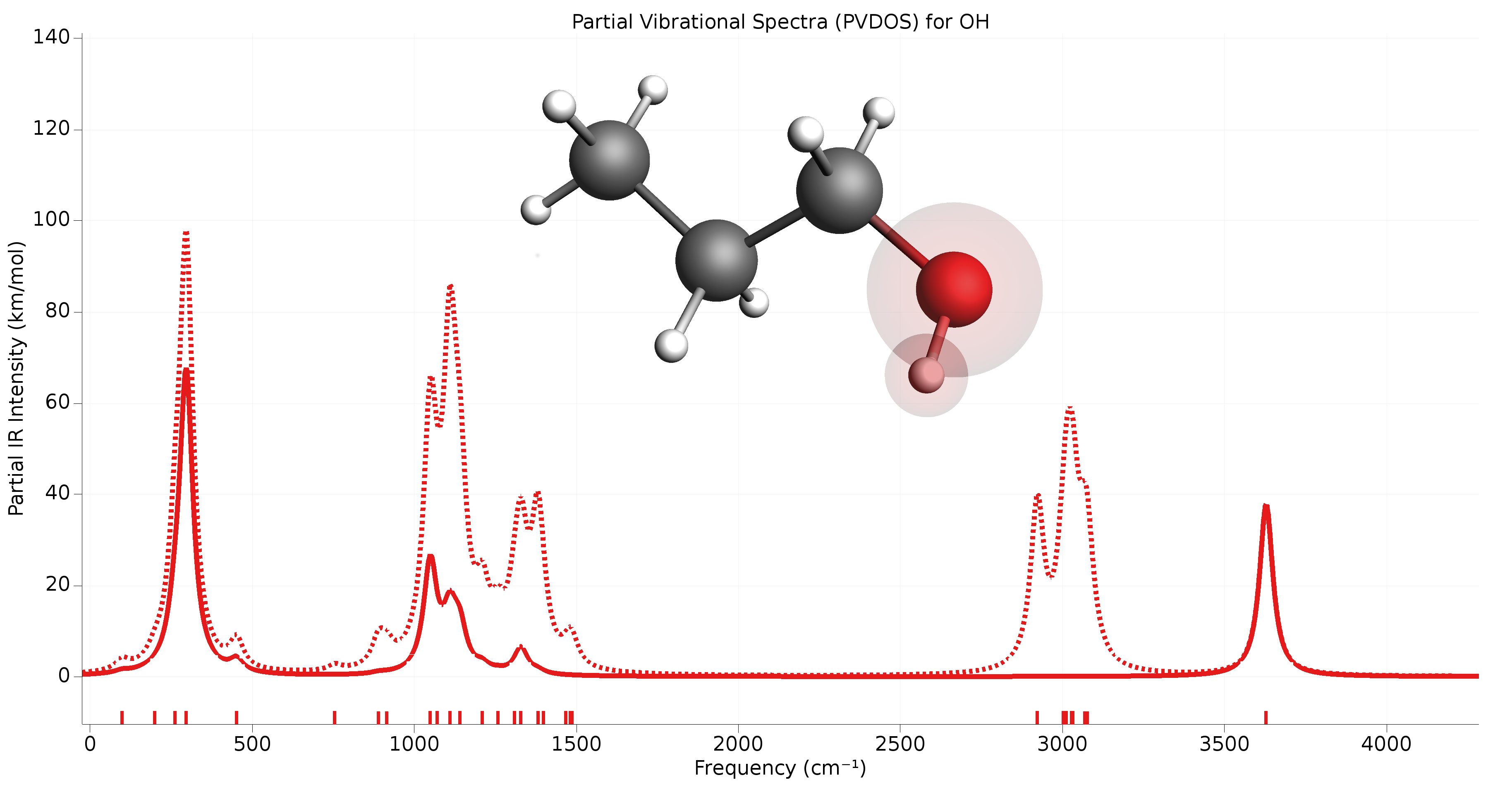
Fig. 2 Example of partial vibrational spectrum (PVDOS). The dotted line is the full IR spectrum of 1-propanol. The solid line is the PVDOS-scaled IR spectrum of the OH group (IR spectrum computed using GFN1-xTB).

The PVDOS matrix is not printed to the text output, but only saved to the engine binary output (.rkf) in the variable Vibrations%PVDOS.

PES point character¶

A PES point can according to the slope and curvature of the PES at that point be classified in the following categories:

A local minimum on the PES with vanishing nuclear gradients and no negative frequencies.
A transition state with vanishing nuclear gradients and exactly one negative frequency, i.e. a first order saddle point on the PES.
A higher order saddle point, i.e. a stationary point on the PES with vanishing nuclear gradients but more than one imaginary frequency.
A non-stationary point on the PES. Here the gradients are non-zero.

This classification can easily be done if both the gradients and the normal modes have already been calculated. However, calculating the full Hessian needed for the entire set of normal modes is very expensive and undesirable if one only wants to know the character of a PES point. The AMS driver can quickly, and without calculating the full Hessian, characterize a PES point into one of the above categories. This can be used to confirm the success of e.g. a transition state search or geometry optimization. A PES point can be characterized by requesting PESPointCharacter as a property:

Properties
   PESPointCharacter [True | False]
End

Properties

PESPointCharacter

Type:	Bool
Default value:	False
GUI name:	Characterize PES point
Description:	Determine whether the sampled PES point is a minimum or saddle point. Note that for large systems this does not entail the calculation of the full Hessian and can therefore be used to quickly confirm the success of a geometry optimization or transition state search.

This will calculate the few lowest normal modes using an iterative diagonalization of the Hessian [1] based on a Davidson algorithm implemented in the PRIMME library [2]. The procedure has been optimized for finding a small number of low-lying eigenvalues in as few matrix-vector multiplications (and thus single point calculations) as possible. This is facilitated by performing the iterative method using a pre-conditioning matrix based on an approximation of the Hessian. The approximate Hessian is obtained from the full Hessian at a lower level of theory. This calculation also provides the initial guesses for the desired normal modes. What the lower level of theory is depends on the main engine used in the calculation: DFTB with the GFN1-xTB model is used as the lower level of theory for relatively slow engines, e.g. DFT based engines. For semi-empirical engines like DFTB or MOPAC, the lower level of theory is currently UFF. It is currently not possible to change the engine used to obtain the preconditioning Hessian and the approximate modes.

Note that the iterative calculation of the normal modes is skipped when …
1. … the nuclear gradients are so large that the PES point is considered non-stationary. The calculation of the modes is then just not necessary for classifying it.
2. … the full normal modes or Hessian have also been requested. The iterative calculation is then not necessary, as all modes are already known.
3. … the molecule is very small. (For small systems the iterative calculation of the few lowest normal modes is not faster than the full calculation of all modes, so all modes are calculated instead.)
The classification as a stationary or non-stationary point uses the gradient convergence criterion from the geometry optimizer as the tolerance, see geometry optimization. This makes sure that the criterion for what is considered converged/stationary is always in sync between the optimizer and the PES point characterization.
For periodic systems the PES point characterization does not take the lattice degrees of freedom into account. A PES point where the nuclear gradients are small enough would for example be classified as a stationary point, even if the system is under stress.

Details of the iterative procedure can be configured in the PESPointCharacter block:

PESPointCharacter
   Displacement float
   NumberOfModes integer
   Tolerance float
End

PESPointCharacter

Type:	Block
Description:	Options for the characterization of PES points.

Displacement

Type:	Float
Default value:	0.04
Description:	Controls the size of the displacements used for numerical differentiation: The displaced geometries are calculated by taking the original coordinates and adding the mass-weighted mode times the reduced mass of the mode times the value of this keyword.

NumberOfModes

Type:	Integer
Default value:	2
Description:	The number of (lowest) eigenvalues that should be checked.

Tolerance

Type:	Float
Default value:	0.02
Description:	Convergence tolerance for residual in iterative Davidson diagonalization.

Note that the residual tolerance that can be achieved is limited by the numerical differentiation that is performed. The default values should apply in most cases, but if convergence becomes a problem one may choose to increase the tolerance or to increase the step size (slightly). Note that the default residual tolerance is lower than for the other mode selective methods. This is because PRIMME uses a different convergence criteria than mode tracking/refinement. The higher value used as a default will therefore not result in decreased levels of accuracy. The method will bail if the number of iterations exceeds the number of normal modes as at this point still achieving convergence becomes unlikely, in part due to the next point.
In order to avoid producing the known and irrelevant rigid modes, the method searches for normal modes orthogonal to six (or five) rigid modes. Imperfections due to the numerical differentiation may mean that the translational and rotational rigid modes are not exact eigenmodes of the Hessian that is constructed. As a result, some part of the lowest vibrational normal mode may lie in the span of the theoretical rigid modes and therefore be inaccessible to the Davidson method. This places a lower bound on the residual tolerance that can be achieved, which is directly related to the numerical differentiation accuracy. The take-away: do not set the tolerance too low, the default usually suffices.
Behind the scenes, the method actually computes a few more modes than requested. In the case of multiplicities, eigenvalues may still converge out of order. These additional eigenvalues essentially guarantee that the obtained modes are indeed the lowest ones.

[1]	Deglmann and F. Furche, Efficient characterization of stationary points on potential energy surfaces, J. Chem. Phys. 117, 9535 (2002)

[2]	Stathopoulos and J. R. McCombs, PRIMME: PReconditioned Iterative MultiMethod Eigensolver: Methods and software description, ACM Transactions on Mathematical Software, Vol. 37, No. 2, (2010), 21:1–21:30.

Elastic tensor¶

The elastic tensor \(c_{\alpha, \beta}\) (Voigt notation) is computed via second order numerical differentiation of the energy \(E\) WRT strain deformations \(\epsilon_\alpha\) and \(\epsilon_\beta\):

\[c_{\alpha, \beta} = \frac{1}{V_0} \frac{\partial^2 E}{\partial \epsilon_\alpha \partial \epsilon_\beta}\]

where \(V_0\) is the volume of the unit cell (for 2D periodic system \(V_0\) is the area of the unit cell, and for 1D periodic system \(V_0\) is the length of the unit cell).

For each strain deformation \(\epsilon_\alpha \epsilon_\beta\), the atomic positions will be optimized. The elastic tensor can be computed for any periodicity, i.e. 1D, 2D and 3D.

Phonons¶

Collective oscillations of atoms around theirs equilibrium positions, giving rise to lattice vibrations, are called phonons. AMS can calculate phonon dispersion curves within standard harmonic theory, implemented with a finite difference method. Within the harmonic approximation we can calculate the partition function and therefore thermodynamic properties, such as the specific heat and the free energy.

Numerical differentiation options¶

The following options apply whenever AMS computes gradients, Hessians or stress tensors via numerical differentiation.

NumericalDifferentiation
   NuclearStepSize float
   StrainStepSize float
   UseSymmetry [True | False]
End

NumericalDifferentiation

Type:	Block
Description:	Define options for numerical differentiations, that is the numerical calculation of gradients, Hessian and the stress tensor for periodic systems.

NuclearStepSize

Type:	Float
Default value:	0.005
Unit:	Bohr
Description:	Step size for numerical nuclear gradient calculation.

StrainStepSize

Type:	Float
Default value:	0.001
Description:	Step size (relative) for numerical stress tensor calculation.

UseSymmetry

Type:	Bool
Default value:	True
Description:	Whether or not to exploit the symmetry of the system for numerical differentiations.

AMS may use symmetry (key NumericalDifferentiation%UseSymmetry) in case of numerical differentiation calculations. If symmetry is used only symmetry unique atoms are displaced. Symmetry is only recognized if the starting geometry has symmetry. Symmetry is only used for molecules if the molecule has a specific orientation in space, like that the z-axis is the main rotation axis. If the GUI is used one can click the Symmetrize button (the star), such that the GUI will (try to) symmetrize and reorient the molecule. There are some cases that even after such symmetrization, the orientation of the molecule is not what is needed for the symmetry to be used in case of numerical differentiation calculations. If that is the case or if key NumericalDifferentiation%UseSymmetry is set to ‘False’, then no symmetry will be used.

The numerical differentiation calculation supports AMS’ double parallelization, which can perform the calculations for the individual displacements in parallel. This is configured automatically, but can be further tweaked using the keys in the NumericalDifferentiation%Parallel block:

NumericalDifferentiation
   Parallel
      nCoresPerGroup integer
      nGroups integer
      nNodesPerGroup integer
   End
End

NumericalDifferentiation

Parallel

Type:	Block
Description:	Numerical differentiation is an embarrassingly parallel problem. Double parallelization allows to split the available processor cores into groups working through all the available tasks in parallel, resulting in a better parallel performance. The keys in this block determine how to split the available processor cores into groups working in parallel.

nCoresPerGroup

Type:	Integer
Description:	Number of cores in each working group.

nGroups

Type:	Integer
Description:	Total number of processor groups. This is the number of tasks that will be executed in parallel.

nNodesPerGroup

Type:	Integer
Description:	Number of nodes in each group. This option should only be used on homogeneous compute clusters, where all used compute nodes have the same number of processor cores.

Other Properties¶

Properties
   DipoleMoment [True | False]
   BondOrders [True | False]
End

Properties

DipoleMoment

Type:	Bool
Default value:	False
Description:	Requests the engine to calculate the dipole moment of the molecule. This can only be requested for non-periodic systems.

BondOrders

Type:	Bool
Default value:	False
Description:	Requests the engine to calculate bond orders. For MM engines these might just be the defined bond orders that go into the force-field, while for QM engines, this might trigger a bond order analysis based on the electronic structure.

Type:	Non-standard block
Description:	Used for the phonon run. The super lattice is expressed in the lattice vectors. Most people will find a diagonal matrix easiest to understand.

Type:	Integer
Default value:	100
Description:	Use interpolation to generate smooth phonon plots.