Vibrational Spectroscopy
General
The starting point is the Hessian of the system, being the second derivative of the energy with respect to the atomic coordinates.
The eigenvalues of the Hessian are the frequencies and the eigen vectors are the normal modes.
As the calculation of the full Hessian is very expensive there are several ways to avoid it, so that you only get a part of the full spectrum, or only modes for a region of the system, see IR frequencies and normal modes section.
A full, partial, or approximate Hessian in itself can be useful for a (Hessian-based) geometry optimization or a transition state search.
Vibrational spectra are obtained by differentiating a property along the normal modes at a (local) minimum of the PES. So for spectra you need to optimize the geometry first, otherwise you get negative frequencies.
The Normal modes and or vibrational spectra can be requested via the Properties block
Properties
   NormalModes Yes/No
   Raman Yes/No
   VROA Yes/No
   VCD Yes/No
   Phonons Yes/No
End
When requesting the normal modes, the IR intensities are calculated, as they are very cheap.
Where are the results?
Because the results of a vibrational spectroscopy calculation are tied to a particular point on the potential energy surface, they are found on the engine output files. Note also that the properties are not always calculated in every PES point that the AMS driver visits during a calculation. By default they are only calculated in special PES points, where the definition of special depends on the task AMS is performing: For a geometry optimization properties would for example only be calculated at the final, converged geometry. This behavior can often be modified by keywords special to the particular running task.
IR frequencies and normal modes
All vibrational Modes
The calculation of the normal modes of vibration can be requested with:
Properties
   NormalModes Yes/No
End
Typically used icw with Task SinglePoint, Task GeometryOptimization, or Task TransitionStateSearch. In case of geometry optimization or transition state search the normal modes will only be calculated at the final, converged geometry.
PropertiesNormalModesType: Bool Default value: No GUI name: Frequencies Description: Calculate the frequencies and normal modes of vibration, and for molecules also the corresponding IR intensities if the engine supports the calculation of dipole moments.
The molecular normal modes are normally calculated within the harmonic oscillation model. If the molecule is in its equilibrium conformation, it sits in the lowest point (at least locally) on the PES. The cross-section of the PES profile close to this point can then be assumed to be approximately parabolic, such that the second derivative of the energy w.r.t a nuclear coordinate can be interpreted as a force constant for the harmonic oscillation of an atom along this coordinate. Since molecular vibrations in polyatomics involve the simultaneous displacement of multiple atoms, this harmonic oscillator model can be generalized to multiple nuclear coordinates. The normal modes and their frequencies then become eigenvectors and eigenvalues of a force constant matrix, the Hessian:
The (non-mass-weighted) Hessian is saved in the engine result file as variable
AMSResults%Hessian. It is not printed to the text output. The column/row
indices are ordered as: x-component of atom 1, y-component of atom 1,
z-component of atom 1, x-component of atom 2, etc.
Most engines cannot calculate the Hessian analytically. The Hessian is then constructed column-wise through numerical differentiation of the energy gradients w.r.t. each nuclear coordinate. AMS will set up 2 single-point calculations (1 for the positive displacement, 1 for the negative displacement), and the requested engine will return the energy gradients at these displacements. These gradients are calculated analytically for most engines.
Note
Numerical calculation of the full Hessian requires 6N single points calculation, which can take a considerable amount of time for large systems. A mode selective method can be a fast alternative, see mode scanning, mode refinement, and mode tracking.
When requesting the normal modes calculation, integrated IR intensities are simultaneously calculated during the finite differentiation steps when constructing the Hessian (as long as dipole moments are supported by the engine). These IR intensities are calculated from the numerical dipole gradients:
Where \(\alpha\) denotes the x-,y- and z-components of the dipole moment \(\mu\), and \(Q^m\) is the mass-weighted vibrational normal mode.
The resulting IR spectrum can be visualized by opening the engine result file with AMSspectra.
The normal modes of vibration and the IR intensities are saved to the
engine result file in the Vibrations section.
Note
The calculation of the normal modes of vibration needs to be done the
system’s equilibrium geometry. So one should either run the normal modes
calculation using an already optimized geometry, or combine both steps into
one job by using the geometry optimization task
together with the Properties%NormalModes keyword.
Symmetry labels of the normal modes may be calculated if AMS uses symmetry in the calculation (key UseSymmetry).
If symmetry is used, the normal modes are projected against symmetric displacements for each irrep. If that is not successful the symmetry label is ‘MIX’.
Symmetry is only recognized if the geometry is (almost) perfectly symmetric and has a specific orientation in space.
You can use the Symmetrize key in the System block to symmetrize and reorient the molecule.
If the AMSinput GUI module is used, one can click the Symmetrize button (the star) and the GUI will try to symmetrize and reorient the molecule.
Rescanning Imaginary modes
The ReScanModes keyword can be used to calculate more accurately frequencies of specific modes
after a normal modes calculation. It is identical to the ScanFreq option
that was available for older versions of ADF and BAND.
Primarily used to identify spurious imaginary modes, and is on by default for this purpose.
See also the Mode Scanning task, which is an extension of this method, but which is not on by default.
NormalModes
   ReScanModes Yes/No
   ReScanFreqRange float_list
End
NormalModesReScanModesType: Bool Default value: Yes GUI name: Re-scan modes Description: Whether or not to scan imaginary modes after normal modes calculation has concluded. ReScanFreqRangeType: Float List Default value: [-10000000.0, 10.0] Unit: cm-1 Recurring: True GUI name: Re-scan range Description: Specifies a frequency range within which all modes will be scanned. 2 numbers: an upper and a lower bound.
Symmetric Displacements
NormalModes
   Displacements Symmetric
End
Specify Displacements Symmetric to calculate the energy Hessian using finite differences in symmetry-adapted displacements, and the corresponding normal modes.
NormalModes
   SymmetricDisplacements
      Type [All | Infrared | Raman | InfraredAndRaman]
   End
End
If Type InfraRed or Type Raman is specified then only irreps that result in non-zero intensities for the corresponding spectroscopy will be included in the calculation.
Using this feature may save a lot of time for large symmetric molecules by skipping calculation of normal modes that would not contribute to the spectrum anyway.
If Type InfraRedAndRaman is specified then vibrations that have a non-zero IR or Raman intensity will be calculated.
If Type All is specified then all vibrations will be calculated. For multi-dimensional irreps (such as E and T) only the first component will be computed.
For any component beyond the first, the frequencies and intensities will be copied from the first one.
NormalModesSymmetricDisplacementsType: Block Description: Configures details of the calculation of the frequencies and normal modes of vibration in symmetric displacements. TypeType: Multiple Choice Default value: All Options: [All, Infrared, Raman, InfraredAndRaman] GUI name: Symm Frequencies Description: For symmetric molecules it is possible to choose only the modes that have non-zero IR or Raman intensity (or either of them) by symmetry. In order to calculate the Raman intensities the Raman property must be requested.
Warning
Specifying Type Raman alone does not trigger calculation of the Raman intensities. In order to calculate the Raman spectrum one should also specify Raman True.
Note
Displacements Symmetric will also produce a 3N-by-3N Hessian matrix but if the Type key’s argument is not All then this matrix will likely have many zero eigenvalues.
Mobile Block Hessian (MBH)
NormalModes
   Displacements Block
End
Specify Displacements Block for the Block Normal Modes option (also known as Mobile Block Hessian, or MBH [1] [2]).
MBH is useful when calculating vibrational frequencies of a small part of a very large system (molecule or cluster). Calculation of the full spectrum of such a system may be inefficient and is unnecessary if one is interested in one particular part. Besides, it may be difficult to extract normal modes related to the interesting sub-system out of the whole spectrum. Using Block Normal Modes it is possible to treat parts of the system as rigid blocks. Each block will usually have only six frequencies related to its rigid motions compared to 3*N for when each atom of the block is treated separately.
MBH is suitable to calculate frequencies in partially optimized structures. Assume a geometry optimization is performed with the Block key in the Constraints input block [see constrained geometry optimizations]. During the geometry optimization, the shape of the block is not changed. The internal geometry of the block is kept fixed, but the block as a whole can still translate or rotate.
At the end of such a partial geometry optimization, the position and orientation of the block is optimized, thus the total force on the block is zero. However, there might be still some residual forces within a block, since those degrees of freedom were not optimized. A traditional frequency calculation performed on this partially optimized structure might result in non-physical imaginary frequencies without a clear interpretation. Therefore one should use an adapted formulation of normal mode analysis: the Mobile Block Hessian method. MBH does not consider the internal degrees of freedom of the block (on which residual forces) apply, but instead uses the position/orientation of the block as coordinates. In the resulting normal mode eigenvectors, all atoms within the same block move collectively.
Of course, MBH can also be applied on a fully optimized structure.
Accuracy
NormalModes
   BlockDisplacements
      AngularDisplacement float
      BlockAtoms integer_list
      BlockRegion string
      Parallel
         nCoresPerGroup integer
         nGroups integer
         nNodesPerGroup integer
      End
      RadialDisplacement float
   End
End
NormalModesBlockDisplacementsType: Block Description: Configures details of a Block Normal Modes (a.k.a. Mobile Block Hessian, or MBH) calculation. AngularDisplacementType: Float Default value: 0.5 Unit: Degree Description: Relative step size for rotational degrees of freedom during Block Normal Modes finite difference calculations. It will be scaled with the characteristic block size. BlockAtomsType: Integer List Recurring: True Description: List of atoms belonging to a block. You can have multiple BlockAtoms. BlockRegionType: String Recurring: True Description: The region to to be considered a block. You can have multiple BlockRegions, also in combination with BlockAtoms. ParallelType: Block Description: Configuration for how the individual displacements are calculated in parallel. nCoresPerGroupType: Integer Description: Number of cores in each working group. nGroupsType: Integer Description: Total number of processor groups. This is the number of tasks that will be executed in parallel. nNodesPerGroupType: Integer GUI name: Cores per task Description: Number of nodes in each group. This option should only be used on homogeneous compute clusters, where all used compute nodes have the same number of processor cores.
RadialDisplacementType: Float Default value: 0.005 Unit: Angstrom Description: Step size for translational degrees of freedom during Block Normal Modes finite difference calculations.
The second derivatives of the energy with respect to Cartesian displacements of the free atoms and those with respect to block motions (3 translation plus 3 rotations) are calculated by numerical differentiation of the gradient. The accuracy of the second derivatives is determined by the accuracy of the gradient evaluation and the step size in the numerical differentiation. The RadialDisplacement and AngularDisplacement parameters can be specified to set the step size for Cartesian displacements (translations) and block rotations respectively. The step size for angles is automatically scaled with the block size.
Note
Blocks should consist of at least 3 atoms (i.e. block of 1 or 2 atoms are not supported).
| [1] | A. Ghysels, D. Van Neck, V. Van Speybroeck, T. Verstraelen and M. Waroquier, Vibrational Modes in partially optimized molecular systems, Journal of Chemical Physics 126, 224102 (2007) |
| [2] | A. Ghysels, D. Van Neck and M. Waroquier, Cartesian formulation of the Mobile Block Hessian Approach to vibrational analysis in partially optimized systems, Journal of Chemical Physics 127, 164108 (2007) |
Mode Scanning
Mode Scanning can be used to obtain more accurate approximations for
properties obtained by numerical differentiation along the vibrational normal modes (frequencies, intensities, Raman, etc.), without changing the modes themselves. Mode Scanning is an extension of the frequency scanning options (ScanFreq) that were part of ADF and BAND in
earlier versions of the Amsterdam Modeling Suite. These latter options are still available as the ReScanModes keyword in the NormalModes block, if these are requested during a calculation.
- Primarily used to identify spurious imaginary modes.
- Improve numerical accuracy of normal mode properties.
- Rescanning modes using a different level of theory.
Theory
Vibrational normal modes are usually obtained as eigenvectors of the Hessian matrix. A common problem with this scheme however, is that due to numerical errors in constructing this Hessian, low-frequency vibrations may be reported to have imaginary frequencies instead. The Mode Scanning task allows for re-calculation of the frequency of these modes. The Mode Scanning task does not change the normal modes itself, only its properties. This Mode Scanning task allows you to confirm whether reported imaginary frequencies are attributed to transition states or whether they are simply due to numerical errors.
Given a user-supplied mode \(Q\), the frequency is calculated from the force constant:
This is again done by numerical differentiation of the energy gradients, requiring AMS to set up 2 single point calculations per selected normal mode. Integrated IR intensities are also calculated simultaneously (if dipole moments are supported by the engine):
Where the derivative is with respect to the mass-weighted normal mode.
It is also possible to use this method to selectively re-calculate the normal mode properties for different engine settings. This has two distinct uses:
- If the modes were originally generated using a finite difference method, a
different stepsize can be used. For strong vibrations (high frequencies),
large stepsizes may cause inaccuracies due to increasing anharmonic
contributions. For weak vibrations (low frequencies) on the other hand,
stepsizes can often be too small. The displacements associated with these
vibrations are small, which can give incorrect sampling of the PES profile.
This should be compensated for by choosing a larger stepsize. The stepsize
can be set using the
Displacementkey. - Users can also recalculate modes using higher levels of theory. Modes generated from a full frequency analysis using e.g. DFTB can be recalculated using e.g. LDA DFT to obtain more realistic integrated IR intensities. The method used for the single point calculations can be set in the Engine block.
Input
A numerical frequency calculation is performed by requesting the
VibrationalAnalysis task with Type ModeScanning:
Task VibrationalAnalysis
VibrationalAnalysis
   Type ModeScanning
   Displacement 0.001
   NormalModes
     ModeFile adf.rkf
     # select all modes with imaginary frequencies
     ModeSelect
        ImFreq true
     End
   End
End
The Mode Scanning tasks uses only the NormalModes block for its input handling. Here, ModeFile specifies the AMS output file containing the normal modes for which you want to calculate the frequencies. The ModeSelect block is used to specify which of the modes in this file should be recalculated, since we are often only interested in a select few of them. A more detailed overview of this block is given in the section Selecting Modes on the main page. Finally, Displacement can be used to specify the stepsize (in Bohr) for the finite differences. The stepsize is provided for displacements along the Cartesian normal modes.
The Mode Scanning module is the main driving force for the Mode Tracking and Vibrational Mode Refinement tasks,
which provide more advanced options for refining not only the properties of the
modes, but also the modes themselves. Consult the relevant pages for more
information. Alternatively, a simplified version of Mode Scanning is available
which follows the old implementation in ADF and BAND (as the ScanFreq option).
This version can be enabled when doing a full frequency analysis by enabling the
Properties%NormalModes keyword. See the
Full Analysis page for further details.
Mode Refinement
With this option you can improve the normal modes, by importing previously calculated modes and then applying a more accurate engine, or more accurate settings, typically for only part of the spectrum. The vibrational Mode Refinement method not only refines frequencies from a previous calculation, but also tries to correct the vibrational modes themselves.
- Refinement of spectral regions requires a sufficient number of modes in the basis to be accurate.
- 1-step refinement. No iterative improvement possible. (Unless followed by a separate Mode Tracking calculation.)
- Quality of the results depends on accuracy of the selected guess modes.
If we start from e.g. a semi-empirical method such as in MOPAC, we can get approximations for the vibrational modes. Mode Refinement then re-calculates part of the Hessian for a subset of these modes using a more accurate method such as GGA DFT, and updates the normal modes themselves to fit this more accurate method. It is intended to circumvent the expensive calculation of the Hessian if you are only interested in a (small) part of the full spectrum. This is based on the method in reference [3].
Because the Mode Refinement method uses linear combinations of the guess modes, its accuracy depends on the set of modes that is supplied.
- If we want to e.g. obtain a mode which includes a C=O stretch, then the initial set must contain a mode which has this C=O stretch, otherwise this cannot be included in the refined modes.
- If we are refining a region containing many similar modes, e.g. vibrations of aromatic ring backbones, and we only use part of this spectral region for the initial set, the set of refined modes will “drift” towards the centre of the spectral region as a results of mode-mixing. This is again an artefact of missing character in the modes.
- This mode-mixing may result in reduced accuracy for some of the modes, as this procedure minimizes the total error for all of the modes. Instead of having a couple of modes with large errors, mode-mixing tends to spread out the error across multiple normal modes. Adding 1 “bad” mode to the basis can then negatively affect your results.
- The advantage of Mode Refinement over Mode Tracking is the ability to refine entire spectral regions at once. If we have a good basis, Mode Refinement can be less computationally expensive than Mode Tracking. If you want to refine larger sections of the spectrum, Mode Refinement is therefore recommended. If you only want to calculate a select few modes, use Mode Tracking to avoid basis dependence and to assure accuracy of the obtained modes.
- For characteristic peaks, Mode Tracking shows very good convergence, and will thus be cheaper to use than Mode Refinement. For (semi-)degenerate modes however, Mode Refinement works better due to the poor tracking performance for these modes.
See also
The GUI tutorial on Mode Refinement.
Theory
We are going to start from a set of normal modes \(b\), obtained from e.g. a semi-empirical or force-field method. First, this task runs the numerical frequency calculation for all selected normal modes, but this time using an ab initio method such as DFT. During the finite difference steps, we also calculate the projection of the Hessian onto the normal modes:
This term is calculated through finite differences on the analytical gradients of the electronic energy along the mass-weighted normal modes \(b^m\). The index \(i\) denotes the \(3N\) nuclear coordinates. These projections are then used to construct a Rayleigh matrix:
Here, \(B^m\) and \(\Sigma\) are matrices containing the \(b^m\) and \(\sigma\) vectors. The eigenvectors of \(\tilde{H}^m\) give us the coefficient series for linear combinations of the normal modes \(b^m\) such that we obtain a new set of modes \(q\):
These modes \(q\) are the closest approximation to the DFT-modes that we could obtain from a linear combination of the approximate modes \(b\). In other words: the approximate modes \(b\) are used as a basis for finding the modes from a more sophisticated theory.
Input
This method inherently features a trade-off:
- The computational benefit comes from only performing the finite difference calculations for the selected modes. By only selecting a small set of modes that we are interested in, we minimize computational expense.
- The more modes we select, the larger the basis for constructing the refined modes. Running for a larger number of modes yields better results. (In the extreme case, running for all 3N modes equates to constructing the full Hessian.)
In practice, Mode Refinement requires you to select a reasonable portion of the spectrum to get accurate results. Specifically, you should select all modes in a region of the spectrum which look similar. Ring structures for instance often feature broad frequency regions with many ring distortions. Even if you are only interested in a couple of these, you should still select all modes in this region, to assure sufficient basis size. Vibrational modes involving ring substituents can however be omitted, which is where we save computation time.
If you are interested only in IR-active vibrations, you could further minimize the basis by only selecting the approximate modes which are IR-active (since adding the non-active modes to the linear expansion does not affect the IR-intensity of the refined modes). Do note that if the semi-empirical method used for calculating the approximate modes yields poor approximations for the dipole gradients, it may be safer to include also modes with very low IR intensity. This is because their low IR-activity may have only been due to the low accuracy of the approximate method.
See also
A tutorial showing this basis representability.
A Mode Refinement calculation is set up by requesting the VibrationalAnalysis
task with the Type ModeRefinement:
Task VibrationalAnalysis
VibrationalAnalysis
   Type ModeRefinement
   Displacement 0.001
   NormalModes
     ModeFile adf.rkf
     ModeSelect
        ...
     End
     ScanModes true
   End
End
The details of the calculation are specified in the NormalModes block.
Here, ModeFile specifies the AMS output file containing the normal modes
for which you want to calculate the frequencies. The ModeSelect block is
used to specify which of the modes in this file will be selected for
refinement. A more detailed overview of this block is given in the section
Selecting modes on the main page. Finally,
Displacement can be used to specify the stepsize (in Bohr) for the finite
differences. The stepsize is provided for displacements along the Cartesian
normal modes.
The ScanModes key in the NormalModes block can be used to
automatically run a numerical frequencies calculation on
the new modes \(q\). Mode Refinement uses a linear combination of modes and
properties, all obtained through finite differences. These results may still
contain some minor errors due to the accumulation of numerical errors from the
linear expansion, or stepsize issues in the numerical frequency calculations.
While commonly not necessary, it is possible to run an additional numerical
refinement calculation on the new modes to minimize these errors. Only in
exceptional cases will these errors be significant. Running this additional
refinement step is therefore only necessary if you need complete certainty that
the results are accurate.
Mode Tracking
The Mode Tracking task is an interface for mode- and intensity-tracking methods, adapted from the MoViPac suite [4]- [5]. These methods can be used to obtain select normal modes, without having to calculate the entire vibrational spectrum. It does this through an iterative procedure.
- Calculations are conducted for each mode separately. Converges fastest for characteristic (non-highly degenerate) modes.
- Iterative approximation to the true modes. Guaranteed to give the correct normal modes if the procedure converges.
- Will not necessarily reproduce the entire spectrum as multiple guess modes can converge to the same normal mode.
Mode Tracking uses information about the known parts of the Hessian to expand its basis iteratively:
- Missing C-O stretch character can thus be recovered in this procedure, and there is no basis dependency.
- For large regions with similar modes however, it is possible that multiple guess modes converge to the same normal mode. Running mode tracking for all modes in this region might not reproduce all unique normal modes.
- The advantage of Mode Refinement over Mode Tracking is the ability to refine entire spectral regions at once. If we have a good basis, Mode Refinement can be less computationally expensive than Mode Tracking. If you want to refine larger sections of the spectrum, Mode Refinement is therefore recommended. If you only want to calculate a select few modes, use Mode Tracking to avoid basis dependence and to assure accuracy of the obtained modes.
- For characteristic peaks, Mode Tracking shows very good convergence, and will thus be cheaper to use than Mode Refinement. For (semi-)degenerate modes however, Mode Refinement works better due to the poor tracking performance for these modes.
Mode Tracking starts with a numerical frequency calculation, which refines the initial guess \(b^m\) for the selected mode. The error of this mode with respect to the true Hessian eigenvector is calculated. This error is used in a (Jacobi-)Davidson algorithm to generate an additional mode. In subsequent iterations, we use these modes as approximations to the true normal modes. In this way, the error of the mode is minimized iteratively, yielding a closer approximation to true normal modes. This is how Mode Tracking differs from the Mode Refinement methods, in that it guarantees that the obtained modes are correct (assuming the procedure has converged).
See also
The GUI tutorial on Mode Tracking.
Theory
During the numerical frequency calculation, we obtain also the projection of the Hessian onto this mode:
This term is calculated through finite differences on the analytical gradients of the electronic energy along the mass-weighted normal modes \(q^m\). The index \(i\) denotes the \(3N\) nuclear coordinates. From this projection a Rayleigh matrix is generated:
Here, \(B^m\) and \(\Sigma\) are matrices containing the \(b^m\) and \(\sigma\) vectors for all foregoing iterations. During each iteration \(k\), if we have not converged, we generate an updated guess vector \(b_k^m\), and so the number of vectors in the matrices above is equal to the number of iterations \(k\). The eigenvectors of \(\tilde{H}^m\) give us the coefficient series for linear combinations of the guess modes \(b^m\) such that we obtain approximations for the true normal modes:
Each iteration, we expand the vector basis \(B^m\), which allows this series expansion to come closer to the true normal modes each time. We can also calculate the error of this mode with respect to how close it is to being an eigenvalue of the real Hessian:
Here, \(\lambda\) is the corresponding eigenvalue of \(\tilde{H}^m\). \(r\) is the residual vector, giving the error for each vector element. It should be zero if the mode is an exact eigenvector of the true Hessian.
Since \(\tilde{H}^m\) may give multiple eigenvectors, several approximate
modes will be generated during those iterations. Out of these, 1 mode is
identified as the mode of interest according to the specified tracking
method. If the residual of this mode has been minimized
sufficiently, the procedure has converged. If not, we generate a new guess
vector \(b_k^m\). There are 2 algorithms for generating this new guess, set
by UpdateMethod in the ModeTracking block:
Davidson method
The Davidson method uses a pre-conditioner \(D\) to generate a new guess mode from the residual vector of the mode selected by the tracking method:
This preconditioner is constructed from an approximation of the Hessian:
The Davidson method works reasonably well, but can have trouble converging if the approximate modes or the Hessian are too accurate. This results as the new vectors that are generated do not necessarily extend the span of the basis. [6]
vdVorst-Sleijpen-Jacobi-Davidson
This variant of the Jacobi-Davidson scheme from Sleijpen & vdVorst [6] automatically makes the new guess vector orthogonal to the normal mode selected by the tracking method:
The new vector is therefore guaranteed to extend the span of the basis as much as possible, and thus also eliminates the aforementioned issue with the Davidson method. In general, it is therefore recommended to use this Jacobi-Davidson method since it is found to converge faster, and be more reliable, as a result of yielding better guess modes.
Input
Task VibrationalAnalysis
VibrationalAnalysis
   Type ModeTracking
   ...
   ModeTracking
      HessianGuess [Unit | File | UFF | Inline]
      HessianInline # Non-standard block. See details.
         ...
      End
      HessianPath string
      UpdateMethod [JD | D | I]
      MaxIterations integer
      ...
      GramSchmidt [True | False]
      GramSchmidtIterations integer
      GramSchmidtTolerance float
   End
End
There are 4 methods to obtain the approximate Hessian \(H_A\), used by both
update methods. They are set by HessianGuess:
HessianGuess [Unit | File | UFF | Inline]UFF- is the default, which generates the approximate Hessian using UFF. While this Hessian may not yield the correct modes by itself, it produces good results as a preconditioner since it correctly represents the molecular structure.
File- will read the Hessian from an AMS output file, which can be
specified in
HessianPath. Using a Hessian from a more advanced method will generally yield better results for the Jacobi-Davidson method. The Davidson method will however experience difficulties with convergence as the Hessian becomes too accurate. [6] Inlinewill read a Hessian specified in the input file, in the
HessianInlineblock. This allows you to use Hessians generated in external programs:Task VibrationalAnalysis VibrationalAnalysis Type ModeTracking ModeTracking HessianGuess Inline # Approximate Hessian for H2O: 3 x nAtoms = 9 so 9x9 Hessian HessianInline 0.62088786 0.00000000 0.00000000 -0.31044393 0.00000000 -0.21902068 -0.31044393 0.00000000 0.21902068 0.00000000 0.00000000 0.00000000 0.00000000 0.00000000 0.00000000 0.00000000 0.00000000 0.00000000 0.00000000 0.00000000 0.32143213 -0.15284008 0.00000000 -0.16071607 0.15284008 0.00000000 -0.16071607 -0.31044393 0.00000000 -0.15284008 0.33598889 0.00000000 0.18593038 -0.02554496 0.00000000 -0.03309030 0.00000000 0.00000000 0.00000000 0.00000000 0.00000000 0.00000000 0.00000000 0.00000000 0.00000000 -0.21902068 0.00000000 -0.16071607 0.18593038 0.00000000 0.15761846 0.03309030 0.00000000 0.00309761 -0.31044393 0.00000000 0.15284008 -0.02554496 0.00000000 0.03309030 0.33598889 0.00000000 -0.18593038 0.00000000 0.00000000 0.00000000 0.00000000 0.00000000 0.00000000 0.00000000 0.00000000 0.00000000 0.21902068 0.00000000 -0.16071607 -0.03309030 0.00000000 0.00309761 -0.18593038 0.00000000 0.15761846 End End End
Unit- uses the unit matrix. This is evidently not a good approximation for the Hessian, and is not intended to be used for proper Mode Tracking runs. However: using a poor approximation for the Hessian can result in basis vectors being generated that we would not obtain otherwise. Running Mode Tracking with this option can allow you to “probe” the vector space to obtain guesses for normal modes, which can be used as starting points for proper Mode Tracking calculations. It is however generally recommended to instead do e.g. a DFTB or UFF run if your goal is to obtain guess modes.
UpdateMethod [JD | D | I]JD- vdVorst-Sleijpen variant of Jacobi-Davidson (Mode tracking default).
D- Davidson
I- No preconditioner (VST default). This is not recommended for typical mode tracking applications, but is useful for a variation of mode tracking, Vibronic-Structure Tracking.
In later iterations, the basis \(B^m\) will become larger. In order to improve the guess modes even further, an iterative Gram-Schmidt procedure is used to orthogonalize the new guess mode to the existing basis. An iterative procedure is necessary to account for numerical noise.
GramSchmidt [True | False]- Expert key. Sets whether to perform this Gram-Schmidt orthogonalization
step. It is
Trueby default. GramSchmidtTolerance float- Expert key. Sets the absolute tolerance for orthogonality of the basis. It is evaluated with respect to the norm of the overlap vector between the new guess mode and the basis of the previous iteration \(||{b_k^m}^T B^m||\).
GramSchmidtIterations- Expert key. Sets the maximum number of allowed iterations during the Gram-Schmidt procedure.
The default settings for the Gram-Schmidt procedure should work for almost all systems.
MaxIterations integer- Finally, the Mode Tracking input block contains the
MaxIterationskey. It sets the maximum allowed number of iterations that the Mode Tracking calculation may go through. If this number is reached, the calculation will stop even if convergence was not achieved. If no value is supplied, a default of \(3N/2\) will be used. This is approximately the maximum number of iterations where the procedure remains computationally competitive with the construction of the full Hessian.
Additional input parameters
Task VibrationalAnalysis
VibrationalAnalysis
   Type ModeTracking
   Displacement float
   ...
   NormalModes
      ScanModes [True | False]
      ...
   End
End
Displacement float- is the displacement stepsize (in Bohr) that is used for calculating frequencies, IR intensities and the Hessian projections through finite differences. The stepsize is provided for displacements along the Cartesian normal modes.
ScanModes [True | False]- key (False by default) in the
NormalModesvibrational analysis sub-block can be used to automatically run a numerical frequencies calculation on the new modes \(Q\) after the Mode Tracking calculation has finished. Ritz vectors are obtained here as linear combinations of the guess modes, which in turn follow from finite difference calculations. This makes it possible for numerical errors to accumulate in the normal modes. Only in exceptional cases will these errors be significant, and running this additional refinement step is therefore only necessary if you need complete certainty that the results are accurate.
Input: Tracking methods
The TrackingMethod parameter allows you to select what property of the
normal modes you want to track. At the end of each iteration, we obtain a set
of approximate normal modes. The tracking method identifies which of these
modes fits best for some criterion, and either returns this mode as the
calculation result, or, if convergence was not achieved, uses it to generating
a new basis mode for the next iteration. In general these methods are
distinguished in 3 categories:
Task VibrationalAnalysis
VibrationalAnalysis
   Type ModeTracking
   ModeTracking
      TrackingMethod [OverlapInitial, DifferenceInitial, FreqInitial, IRInitial,
                      OverlapPrevious, DifferencePrevious, FreqPrevious, IRPrevious,
                      HighestFreq, HighestIR, LowestFreq, LowestResidual]
      ...
   End
End
Mode Tracking
The original tracking methods focus on obtaining as accurate as possible a normal mode for the system. This class of tracking methods focuses either on accuracy of the mode, or obtaining modes with particular vibrational character:
TrackingMethod [OverlapInitial, DifferenceInitial, FreqInitial, OverlapPrevious, DifferencePrevious, FreqPrevious, HighestFreq, LowestFreq, LowestResidual]OverlapInitial- is the default tracking method. Here, we choose the mode which resembles most closely the guess mode that was initially supplied \(b_1^m\). This is done by choosing the mode which has the greatest overlap with the initial guess vector. This method allows us to direct the optimization towards modes that e.g. involve particular atoms or include particular bending/stretching vibrations.
OverlapPrevious- instead chooses the mode which resembles closest the
approximate mode of the previous iteration \(Q_k^m\). This procedure
allows a bit more flexibility in the optimization. Since we essentially
“forget” about earlier iterations, this procedure allows the optimization to
correct errors in the initial guess. (It is possible for instance that the
initial guess included 2 different bond stretches which do not mutually occur
in the true modes. This method will then converge quicker to a mode involving
only 1 of these stretches, whereas
OverlapInitialwill take a much larger number of iterations to achieve this, if it does so at all.) Do note that this means that the final mode that you obtain does not necessarily represent the mode you initially supplied. DifferenceInitial- works the same as
OverlapInitial, except that it chooses the mode which has the smallest norm for the difference vector between the initial mode and the approximate normal modes of this iteration. The use of the difference vector prioritizes deviations in the dominant parts of the vibrational character. E.g. if a mode consists primarily of a CO stretch, plus some minor vibrations in a carbon backbone, it may be desired to prioritize getting the correct force constant for the dominant CO stretch. This is achieved using these difference vector methods. In general, overlap methods still work well in these situations, and the use of difference methods should only be necessary in extreme cases. DifferencePrevious- is also the same as
DifferenceInitialexcept for the use of the difference vector norm as the selection criterion. FreqInitial- chooses the mode with the frequency closest to that of the initial guess. This allows us to direct the tracking towards modes in a particular frequency region of the spectrum. Note that convergence for these frequency-based methods is slightly slower since the character of the mode itself is not included in the selection criteria, allowing for larger differences in the modes between iterations.
FreqPrevious- is similar to
FreqInitialexcept that we choose the mode with the frequency closest to that of the previous iteration. This allows the optimization more freedom to move away from the frequency region of the initial guess, and thus allows to correct somewhat for poor initial guesses. HighestFreq- chooses the mode with the highest frequency. This method can be used if it is desired to track particular characteristic high-frequency vibrations.
LowestResidual- chooses the mode which has the smallest norm for the residual vector (see the ‘Convergence’ section below.) This method only focuses on obtain the most accurate mode, regardless of vibrational character or where it lies in the spectrum. This method should generally only be used as a pre-conditioner if you have very little information on what the normal modes should look like. (Since it is basically a non-directed optimization.) This method will then try and find the normal mode closest to your guess. The approximate normal mode obtained this way will most likely not have converged yet, but should give you an indication of what the normal modes may look like. You can use these modes to refine your initial guess, and then do a new Mode Tracking run using any of the other tracking parameters to obtain the desired mode. Although this strategy is possible, it is generally recommended to use an approximate method to get an initial guess for the normal modes instead (as shown in the examples).
Intensity Tracking
This class of methods focuses on tracking modes based on their intensity in e.g. the infrared spectrum, rather than focusing on getting a mode with a particular type of vibration.
TrackingMethod [IRInitial, IRPrevious, HighestIR]IRInitialchooses the mode with the IR intensity closest to that of the initial guess. This constrains the optimization to modes which are IR active, a property that may be lost when using mode tracking update methods.IRPrevioussimilarly chooses the mode with the IR intensity closest to that of the previous iteration. This allows the method some more flexibility in varying the intensity of the vibration, and thus works better if the initial guess is not that good.HighestIRchooses the mode with the highest IR intensity. This option can be used to find the modes associated with sharp peaks in the IR spectrum.
With Intensity Tracking, we essentially add an additional requirement to the modes: they must have a particular IR intensity. This constrained search has different convergence characteristics than conventional mode tracking, which you should take into account when setting up the mode tracking calculations.
- The majority of modes will have near-zero IR intensity. If we use a near-zero
IR intensity mode as our initial guess, and request
IRIntitialorIRPrevious, then we could be tracking any of one of these. Conversely, convergence behavior will be poor since the generated basis modes are essentially random. If you are trying to obtain a high IR-intensity mode, use an IR-susceptible mode.
Note
In our conventional work-flow, we recommend starting mode tracking or
refinement calculations from a set of approximate normal modes obtained from
a semi-empirical or force-field method. Note however, that these method often
do not produce accurate IR intensities. When selecting the initial guess
mode, do not use the IRRange or related options in the ModeSelect
block. This will cause you to miss vibrations which were incorrectly labeled
with low IR intensity, or vice versa. Instead, rely on chemical intuition to
identify the modes which contain commonly IR active vibrational components
(such as C-O or N-H stretches). You can use AMSspectra in the GUI to
visualize the vibrational modes, to help you in this process.
- To allow the intensity tracking procedure to converge faster, it is
recommended to use the
IRPrevioustag instead of theIRInitialtag. As discussed earlier, the former allows more flexibility in the optimization procedure, which counters the rigidity imposed by the intensity constraint. Intensity tracking methods often need this additional flexibility in generating guess modes to converge to the desired modes. - Poor Initial Guesses: During each iteration, we still use the mode tracking methods to generate new basis modes. These basis modes try to expand the span of the basis with respect to the vibrational character of the modes. Note that this expansion does not guarantee that we will expand the basis specifically in the sub-span of IR-susceptible vibrations. If the initial guess for intensity tracking is correct, we already start our search in the sub-span vicinity of the normal modes. Basis expansion is then more efficient and there is a high chance that new guess modes sample the IR characteristic vibrations. For intensity tracking it is therefore discouraged to use poor initial guess modes.
HighestIRis considered a “pure” intensity tracking method, in that it is used specifically to target characteristics of the IR spectrum irrespective of the underlying vibrational character. Consequently, the normal mode character can vary a lot between iterations. In order to assure that the procedure converges to the desired modes, it is recommended to use sufficiently strict tolerances (see the Convergence section). If the tolerances are too lax, the program may consider the modes to be “good enough” based on residual minimization, even though there may be another mode with a higher IR intensity. For this reason it is generally recommended to useToleranceForNormvalues 1 order of magnitude lower than the default, or around0.00005.
Input: Selecting modes
It is possible to track multiple modes in a single Mode Tracking calculation. The Mode Tracking task will then run the Mode Tracking algorithm for each mode in order.
The initial guess for the mode which will be tracked can be supplied in several
ways. This is governed by ModeInputFormat:
Task VibrationalAnalysis
VibrationalAnalysis
   Type ModeTracking
   NormalModes
      ModeInputFormat [File | Inline | Hessian]
      ModeFile string
      ModeInline # Non-standard block. See details.
         ...
      End
      ModeSelect
         ...
      End
      MassWeighInlineMode [True | False]
  End
End
ModeInputFormat [File | Inline | Hessian]Inlinewill make the module read the mode from the input file. If this option is selected, you can supply the mode in the
ModeInlineblock. It is possible to supply multiple modes by adding additionalModeInlineblocks. The modes are given with one line for the x,y,z-displacement per atom, and in the same order, as theAtomsblock inSystem:ModeTracking TrackedMode Inline ModeInline 0.00000000 0.00000000 -0.03815965 -0.18888544 0.00000000 0.30281066 0.18888544 0.00000000 0.30281066 End ModeInline 0.00000000 0.00000000 -0.02243153 0.32132452 0.00000000 0.17800237 -0.32132452 0.00000000 0.17800237 End ... End
File- will make the module read modes from an AMS or engine output file,
specified by
ModePath. Modes generated using DFTB can be read from thedftb.rkffile and optimised using Mode Tracking for example. When this option is selected, all the vibrational modes present in the file are read first. TheModeSelectblock then specifies for which of these modes you want to perform the Mode Tracking calculation. Hessian- will generate modes as the eigenvectors of the approximate Hessian
selected for the preconditioner in
HessianGuess. This also allows modes to be generated for Hessians obtained from external programs.ModeSelectspecifies which of the generated vibrational modes are selected for Mode Tracking.
- Settings for the
ModeSelectblock are discussed on the main page.
MassWeighInlineMode [True | False]- decides whether the initial guess modes need to be
mass-weighted (default True). As discussed above, Mode Tracking uses mass-weighted normal
modes. In most cases, the normal modes are given in regular Cartesian
coordinates however. By setting
MassWeighInlineMode true, these Cartesian modes are converted into mass-weighted modes by the program. If you supply a mass-weighted mode through theModeInlineblock however, you do not need the program to do the mass-weighing, and you should setMassWeighInlineMode false.
Input: Convergence
Task VibrationalAnalysis
VibrationalAnalysis
   Type ModeTracking
   ModeTracking
      ToleranceForNorm float
      ToleranceForResidual float
      ToleranceForBasis float
   End
End
In order to guide the Mode Tracking procedure, several convergence criteria are used:
ToleranceForNorm float- is the absolute tolerance for convergence of the norm of
the residual vector. The residual vector is a vector containing the error for
each element of the normal mode, and we use the norm as a measure for the
total error. If the total error is smaller than this threshold, we consider
the mode to be a true normal mode and we stop iterating. Since the value of
this norm depends on the length of the residual vector hence the number of
atoms in the system, this tolerance is scaled internally to the number of
atoms.
0.0005is used as a default value for which most systems will converge to reasonably accurate modes in not too many iterations. If you want a more accurate approximation, you can decrease this value by e.g. 1 order of magnitude. (Consider running using the default settings, and reading the norm at convergence from the logfile. The new norm can be chosen to be lower than this value to ‘force’ the method into another iteration.) ToleranceForResidual float- is the absolute tolerance for the maximum component of the residual vector. Particularly in larger systems, where the vibration may be dominated by a small number of atoms, the error associated with the vibration of the majority of atoms may be small (the scaled residual norm will be small). The error for the atoms involved in the vibration may be comparatively large then, which is why we also check convergence for the maximum component of the error. Note that both the norm and this max. error are checked simultaneously. By varying strictness of the criteria for the norm and the max. error separately, you can prioritize either the total vibration or more localized character.
ToleranceForBasis float- checks that the basis mode generated in the previous iteration, through the (Jacobi-)Davidson method, contributes to the approximate normal mode. Since the approximate mode is taken as a linear combination of the basis modes, its linear expansion coefficient must be larger than this tolerance.
The iterative procedure is stopped in one of two cases. Either both the residual
criteria are achieved, in which case the mode is deemed to be converged and
the program exits normally. Alternatively, the basis criterion is met in which
case a warning is broadcast indicating that the desired level of accuracy of the
mode may not have been reachd yet, but the basis has stopped expanding.
The default values for these parameters should be applicable for most
cases, but can be adjusted if needed. If stricter criteria are required, it is
recommended to adjust both ToleranceForNorm and ToleranceForResidual.
References
| [3] | T.Q. Teodoro, M.A.J. Koenis, S.E. Galembeck, V.P. Nicu, W.J. Buma, L. Visscher, A frequency range selection method for vibrational spectra, J. Phys. Chem. Lett., 9 (23), 6878 (2018) |
| [4] | T. Weymuth, M.P. Haag, K. Kiewisch, S. Luber, S. Schenk, C.R. Jacob, C. Herrmann, J. Neugebauer, M. Reiher, MoViPac: Vibrational Spectroscopy with a Robust Meta-Program for Massively Parallel Standard Inverse Calculations, Journal of Computational Chemistry 33, 2186 (2012) |
| [5] | S. Luber, J.Neugebauer, M. Reiher, Intensity tracking for theoretical infrared spectroscopy of large molecules, Journal of Chemical Physics 130, 064105 (2009) |
| [6] | (1, 2, 3) G.L.G. Sleijpen, H.A. van der Vorst, A Jacobi-Davidson Iteration Method for Linear Eigenvalue Problems, SIAM Journal on Matrix Analysis and Applications 17, 401 (1996) |
Selecting modes
Mode Scanning, Mode Refinement and Mode Tracking as well as VG-FC Vibronic-Structure, VG-FC Vibronic-Structure Refinement and VG-FC resonance Raman all require a set of normal modes to operate on. For Mode Scanning these are the modes that you want to calculate the properties of, for Mode Refinement these modes form the basis modes, and for Mode Tracking these are the initial guess modes. For the VG-FC based methods these modes are the modes responsible for the vibronic coupling to the electronic excitation (in VG-FC Vibronic-Structure Refinement they are refined first).
Note
VG-FC Vibronic-Structure Tracking does not require any normal modes and as such does not
support the ModeSelect (nor does it support the NormalModes block for that matter).
These methods provide options to load a large set of modes, after which the
program will filter out the modes of interest. This is done according to the
keys set in the ModeSelect block.
Note
The ModeSelect block is part of the NormalModes block of the Vibrational
Analysis input. All Vibrational Analysis methods share this block, with the
exception of VG-FC Vibronic-Structure Tracking. The methods for obtaining the
set of modes that we will filter can differ per method. Particularly Mode Tracking
features a lot of additional options, and the vibronic variants feature
more specialized options.
Below is an overview of all the available options for the ModeSelect block
as they appear in the basic vibrational analysis tools. The vibronic variants
are discussed in more detail on their respective documentation pages.
The options below are not mutually exclusive.
ModeSelect
   DisplacementBound float
   FreqAndIRRange float_list
   FreqRange float_list
   Full Yes/No
   HighFreq integer
   HighIR integer
   IRRange float_list
   ImFreq Yes/No
   LargestDisplacement integer
   LowFreq integer
   LowFreqNoIm integer
   LowIR integer
   ModeNumber integer_list
End
ModeSelectDisplacementBoundType: Float Description: Vibronic Structure (Refinement), Resonance Raman: Select all modes with a dimensionless oscillator displacement greater than the specified value. FreqAndIRRangeType: Float List Unit: cm-1 and km/mol Recurring: True Description: Specifies a combined frequency and IR intensity range within which all modes will be selected. First 2 numbers are the frequency range, last 2 numbers are the IR intensity range. FreqRangeType: Float List Unit: cm-1 Recurring: True Description: Specifies a frequency range within which all modes will be selected. 2 numbers: an upper and a lower bound. Calculating all modes higher than some frequency can be achieved by making the upper bound very large. FullType: Bool Default value: No GUI name: All modes Description: Select all modes. This only make sense for Mode Scanning calculations. HighFreqType: Integer GUI name: # High frequencies Description: Select the N modes with the highest frequencies. HighIRType: Integer GUI name: # High IR Description: Select the N modes with the largest IR intensities. IRRangeType: Float List Unit: km/mol Recurring: True Description: Specifies an IR intensity range within which all modes will be selected. 2 numbers: an upper and a lower bound. ImFreqType: Bool Default value: No GUI name: All imaginary frequencies Description: Select all modes with imaginary frequencies. LargestDisplacementType: Integer Description: Vibronic Structure (Refinement), Resonance Raman: Select the N modes with the largest VG-FC displacement. LowFreqType: Integer GUI name: # Low frequencies Description: Select the N modes with the lowest frequencies. Includes imaginary modes which are recorded with negative frequencies. LowFreqNoImType: Integer GUI name: # Low positive frequencies Description: Select the N modes with the lowest non-negative frequencies. Imaginary modes have negative frequencies and are thus omitted here. LowIRType: Integer GUI name: # Low IR Description: Select the N modes with the smallest IR intensities. ModeNumberType: Integer List GUI name: Mode numbers Description: Indices of the modes to select.
Thermodynamics (ideal gas)
The following thermodynamic properties are calculated by default whenever normal modes are computed: entropy, internal energy, constant volume heat capacity, enthalpy and Gibbs free energy. Translational, rotational and vibrational contributions are calculated for entropy, internal energy and constant volume heat capacity.
The results are written to the output file (section: “Statistical Thermal Analysis”) and to the engine binary results file (section: “Thermodynamics”).
The thermodynamic properties are computed assuming an ideal gas, and electronic contributions are ignored. The latter is a serious omission if the electronic configuration is (almost) degenerate, but the effect is small whenever the energy difference with the next state is large compared to the vibrational frequencies. The thermal analysis is based on the temperature dependent partition function. The energy of a (non-linear) molecule is (if the energy is measured from the zero-point energy)
The summation is over all harmonic \(\nu_j\), \(h\) is Planck’s constant and \(D\) is the dissociation energy
Contributions from low (less than 20 1/cm) frequencies to entropy, heat capacity and internal energy are excluded from the total values, but they are listed separately (so the user can add them if they wish).
As an alternative to outright excluding low-frequency contributions, a correction scheme is available that is based on interpolating between harmonic oscillator and free rotor values [7] [8] (Li/Head-Gordon and Grimme). It can greatly reduce the impact of the inaccuracies of the harmonic oscillator model on thermodynamic properties at these low frequencies. The scheme corrects vibrational contributions to entropies, internal energies and constant volume heat capacities. This correction is applied automatically and its results are printed separately (in the text output, the corrected terms are marked with the symbol (c)). When applied, the correction considers all real frequencies, including those less than 20 1/cm.
The interpolation for a corrected thermodynamic property \(f\) at pressure \(p\) and temperature \(T\) in terms of harmonic oscillator terms \(f_{HO}\), free rotor terms \(f_{FR}\), and interpolator terms \(x\) for each harmonic oscillator frequency \(\nu_j\) is:
Where \(\alpha\) is an arbitrary exponent and \(\nu_0\) is the harmonic oscillator frequency around which \(x\) interpolates, with \(x=0.5\) when \(\nu_j=\nu_0\) and \(x\approx1.0\) when \(\nu_j\gg\nu_0\). While the free rotor terms used for internal energies and heat capacities are the standard ones, the terms used for entropies have to use the rotors’ moments of inertia \(\mu_{FR}\) and symmetry \(\sigma\), which formally cannot be calculated from harmonic frequencies alone. The correction scheme instead estimates each moment of inertia as being of a \(\sigma=1\) free rotor whose first excited state has an energy equal to the given \(h\nu_{j}\). After this, each obtained moment of inertia \(\mu_{FR}\) is modified by an averaging moment of inertia \(\mu_{av}\) to avoid grossly overestimating entropies at very small frequencies (less than around 1 1/cm):
Input options
Thermo
   Temperatures float_list
   Pressure float
   LowFrequencyCorrector
      Alpha float
      Frequency float
      MomentOfInertia float
   End
End
ThermoType: Block Description: Options for thermodynamic properties (assuming an ideal gas). The properties are computed for all specified temperatures. TemperaturesType: Float List Default value: [298.15] Unit: Kelvin Description: List of temperatures at which the thermodynamic properties will be calculated. PressureType: Float Default value: 1.0 Unit: atm Description: The pressure at which the thermodynamic properties are computed. LowFrequencyCorrectorType: Block Description: Options for the dampener-powered free rotor interpolator that corrects thermodynamic quantities for low frequencies. See DOI:10.1021/jp509921r and DOI:10.1002/chem.201200497. AlphaType: Float Default value: 4.0 Description: The exponent term used in the dampener. FrequencyType: Float Default value: 100.0 Unit: cm-1 Description: The frequency around which the dampener interpolates between harmonic oscillator and free rotor quantities. MomentOfInertiaType: Float Default value: 1e-44 Unit: kg m^2 GUI name: Averaging Moment of Inertia Description: The moment of inertia used to restrict entropy results for very small frequencies (generally around less than 1 cm-1).
| [7] | Yi-Pei Li, Joseph Gomes, Shaama Mallikarjun Sharada, Alexis T. Bell, Martin Head-Gordon, Improved Force-Field Parameters for QM/MM Simulations of the Energies of Adsorption for Molecules in Zeolites and a Free Rotor Correction to the Rigid Rotor Harmonic Oscillator Model for Adsorption Enthalpies, J. Phys. Chem. C 2015, 119, 4, 1840-1850 |
| [8] | Stefan Grimme, Supramolecular Binding Thermodynamics by Dispersion‐Corrected Density Functional Theory, Chem. Eur. J., 18: 9955-9964 |
Gibbs free energy change for a gas phase reaction
Here an example is given how to calculate the free energy change for a reaction. In the AMS output of a normal modes calculation you can find the electronic bonding energy and nuclear kinetic energies, at room temperature. Example part of the AMS output of a nonlinear molecule:
Zero-point energy (Hartree):     0.0333

...
...

Temp                                                        Transl      Rotat     Vibrat     Total
----                                                        ------      -----     ------     -----

298.15   Entropy (cal/mol-K):                              34.441     11.474      0.137     46.052
         Nuclear Internal Energy (kcal/mol):                0.889      0.889     20.941     22.718
         Constant Volume Heat Capacity (cal/mol-K):         2.981      2.981      0.565      6.526

 Summary of energy terms
                                              hartree              eV         kcal/mol           kJ/mol
                                 --------------------     -----------       ----------      -----------
 Energy from Engine:               -0.743995039793930        -20.2451          -466.86         -1953.36
 Nuclear Internal Energy:           0.036203917534227          0.9852            22.72            95.05
 Internal Energy U:                -0.707791122259703        -19.2599          -444.14         -1858.31
 pV/n = RT:                         0.000944186013486          0.0257             0.59             2.48
 Enthalpy H:                       -0.706846936246217        -19.2343          -443.55         -1855.83
 -T*S:                             -0.021880868282982         -0.5954           -13.73           -57.45
 Gibbs free energy:                -0.728727804529199        -19.8297          -457.28         -1913.27
The Energy from Engine = -466.86 kcal/mol. It depends on the engine how this energy is calculated. In the ADF and BAND engines the energy is normally calculated with respect to (artificial) spherical averaged neutral atoms.
The Nuclear Internal Energy = zero point energy + 3 kT + small correction term = 22.72 kcal/mol. 3 kT = 3/2 kT for rotation, and 3/2 kT for translation (i.e. 1/2 kT for each degree of freedom). The small correction term is a term due to the vibration partition function, depending on the temperature not only the ground state vibrational levels are occupied, see also the previous discussion.
The Internal Energy U = Energy from Engine + Nuclear Internal Energy = -466.86 + 22.72 = -444.14 kcal/mol. Gas phase pV/n = RT = 8.314472 * 298.15 / 4184 = 0.59 kcal/mol. The enthalpy H = U + pV = -444.14 + 0.59 = -443.55 kcal/mol. The Gibbs free energy G = H - TS = -443.55 - 298.15*46.052/1000 = -457.28 kcal/mol.
For a calculation of the free energy change for reaction (\(\Delta\) G), you will have to do this for the reactant and product molecules, and add and subtract these energies, for each molecule proportional to the number of molecules that take place in the reaction. Application of ADF for obtaining enthalpy, entropy and Gibbs free energy can for instance be obtained in Refs. [9] [10].
| [9] | M. Swart, E. Rösler, and F. M. Bickelhaupt, Proton affinities of maingroup-element hydrides and noble gases: Trends across the periodic table, structural effects, and DFT validation, Journal of Computational Chemistry 27, 1486 (2006) |
| [10] | M. Swart, and F. M. Bickelhaupt, Proton Affinities of Anionic Bases: Trends Across the Periodic Table, Structural Effects, and DFT Validation, Journal of Chemical Theory and Computation 2, 281 (2006). |
Moments of inertia
In case normal modes are computed in AMS, AMS also reports the moments of inertia of the molecule in units of amu bohr2 (amu = atomic mass unit) and its corresponding principal axes.
Partial Vibrational Spectra (PVDOS)
The Partial Vibrational Spectra (also known as PVDOS) is computed by default whenever normal modes are requested. The PVDOS \(P_{I,n}\) for atom \(I\) and normal mode \(n\) is defined as:
where \(m_I\) is the nuclear weight of atom \(I\), and \(\vec{\eta}_{I,n}\) is the displacement vector for atom \(I\) in normal normal mode \(n\).
Tip
The Partial Vibrational Spectra (PVDOS) can be visualized using the AMSspectra GUI module (Vibrations → Partial Vibrational Spectra (PVDOS)). When plotting a partial vibrational spectrum, the IR intensity of normal modes is scaled by the corresponding PVDOS of the selected atoms.
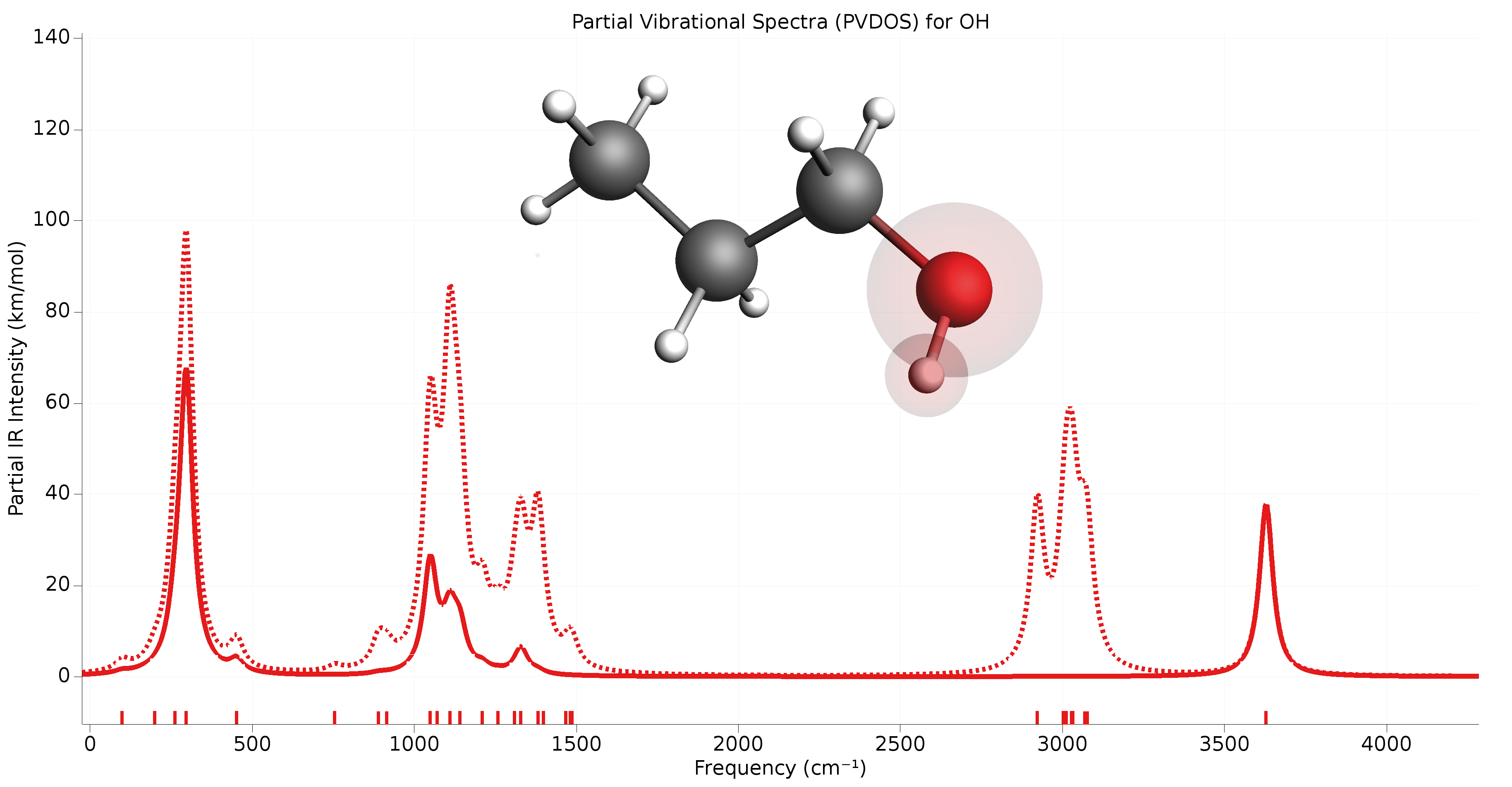
Fig. 2 Example of partial vibrational spectrum (PVDOS). The dotted line is the full IR spectrum of 1-propanol. The solid line is the PVDOS-scaled IR spectrum of the OH group (IR spectrum computed using GFN1-xTB).
The PVDOS matrix is not printed to the text output, but only saved to the engine
binary output (.rkf) in the variable Vibrations%PVDOS.
Phonons
Collective oscillations of atoms around theirs equilibrium positions, giving rise to lattice vibrations, are called phonons. AMS can calculate phonon dispersion curves within standard harmonic theory, implemented with a finite difference method. Within the harmonic approximation we can calculate the partition function and therefore thermodynamic properties, such as the specific heat and the free energy.
See also
Example: Phonons for graphene, Example: Phonons with isotopes, Example: User-defined Brillouin zone for phonon dispersion and diamond lattice optimization and phonons tutorial
The calculation of phonons is enabled in the Properties block.
Properties
   Phonons Yes/No
End
Note
Phonon calculations should be performed on optimized geometries, including the lattice vectors. This can be done by either using an already optimized system as input, or by combining the phonon calculation with the geometry optimization task (you should set the GeometryOptimization%OptimizeLattice input option to True).
The details of the phonon calculations are configured in the
NumericalPhonons block:
NumericalPhonons
   SuperCell # Non-standard block. See details.
      ...
   End
   StepSize float
   DoubleSided Yes/No
   Interpolation integer
   NDosEnergies integer
   AutomaticBZPath Yes/No
   BZPath
      Path # Non-standard block. See details.
         ...
      End
   End
   Parallel
      nCoresPerGroup integer
      nGroups integer
      nNodesPerGroup integer
   End
End
NumericalPhononsSuperCellType: Non-standard block Description: Used for the phonon run. The super lattice is expressed in the lattice vectors. Most people will find a diagonal matrix easiest to understand.
The most important setting here is the super cell transformation. In principle this should be as large as possible, as the phonon bandstructure converges with the size of the super cell. In practice one may want to start with a 2x2x2 cell and increase the size of the super cell until the phonon band structure converges:
NumericalPhonons
   SuperCell
      2 0 0
      0 2 0
      0 0 2
   End
End
By default the phonon dispersion curves are computed for the standard path though the Brillouin zone (see https://doi.org/10.1016/j.commatsci.2010.05.010). One can request the a different path using the following keywords (for an example of how to specify a user-defined path see Example: User-defined Brillouin zone for phonon dispersion):
NumericalPhonons
   AutomaticBZPath Yes/No
   BZPath
      Path # Non-standard block. See details.
         ...
      End
   End
End
NumericalPhononsAutomaticBZPathType: Bool Default value: Yes GUI name: Automatic BZ path Description: If True, compute the phonon dispersion curve for the standard path through the Brillouin zone. If False, you must specify your custom path in the [BZPath] block. BZPathType: Block Description: If [NumericalPhonons%AutomaticBZPath] is false, the phonon dispersion curve will be computed for the user-defined path in the [BZPath] block. You should define the vertices of your path in fractional coordinates (with respect to the reciprocal lattice vectors) in the [Path] sub-block. If you want to make a jump in your path (i.e. have a discontinuous path), you need to specify a new [Path] sub-block. PathType: Non-standard block Recurring: True Description: A section of a k space path. This block should contain multiple lines, and in each line you should specify one vertex of the path in fractional coordinates. Optionally, you can add text labels for your vertices at the end of each line.
Other keywords in the NumericalPhonons block modify the details of the numerical differentiation
procedure and the accuracy of the results:
NumericalPhononsStepSizeType: Float Default value: 0.04 Unit: Angstrom Description: Step size to be taken to obtain the force constants (second derivative) from the analytical gradients numerically. DoubleSidedType: Bool Default value: Yes Description: By default a two-sided (or quadratic) numerical differentiation of the nuclear gradients is used. Using a single-sided (or linear) numerical differentiation is computationally faster but much less accurate. Note: In older versions of the program only the single-sided option was available. InterpolationType: Integer Default value: 100 Description: Use interpolation to generate smooth phonon plots. NDosEnergiesType: Integer Default value: 1000 Description: Nr. of energies used to calculate the phonon DOS used to integrate thermodynamic properties. For fast compute engines this may become time limiting and smaller values can be tried.
The numerical phonon calculation supports AMS’ double parallelization, which can perform the calculations for the individual displacements in parallel. This is configured automatically, but can be further tweaked using the keys in the NumericalPhonons%Parallel block:
NumericalPhonons
   Parallel
      nCoresPerGroup integer
      nGroups integer
      nNodesPerGroup integer
   End
End
NumericalPhononsParallelType: Block Description: Options for double parallelization, which allows to split the available processor cores into groups working through all the available tasks in parallel, resulting in a better parallel performance. The keys in this block determine how to split the available processor cores into groups working in parallel. nCoresPerGroupType: Integer GUI name: Cores per group Description: Number of cores in each working group. nGroupsType: Integer GUI name: Number of groups Description: Total number of processor groups. This is the number of tasks that will be executed in parallel. nNodesPerGroupType: Integer GUI name: Nodes per group Description: Number of nodes in each group. This option should only be used on homogeneous compute clusters, where all used compute nodes have the same number of processor cores.
(Resonance) Raman
Raman
In this method the Raman scattering spectrum is calculated from the geometrical derivatives of the frequency-dependent polarizability. Engine ADF is required. Raman scattering intensities and depolarization ratios for all or a selected number of molecular vibrations at a certain laser frequency can be calculated. The Raman scattering calculation is very similar to an IR intensity calculation. In fact, all IR output is automatically generated as well. At all distorted geometries the dipole polarizability tensor is calculated. This is time-consuming and is only feasible for small molecules.
Properties
   Raman Yes/No
End
Raman
   IncidentFrequency float
   FreqRange float_list
End
If a FreqRange is included the Raman intensities are calculated for a range of vibrational frequencies only.
Using this option is a fast alternative for calculating all Raman intensities.
PropertiesRamanType: Bool Default value: No Description: Requests calculation of Raman intensities for vibrational normal modes.
RamanIncidentFrequencyType: Float Default value: 0.0 Unit: eV Description: Frequency of incident light. FreqRangeType: Float List Unit: cm-1 Recurring: True GUI name: Frequency range Description: Specifies a frequency range within which all modes will be scanned. 2 numbers: an upper and a lower bound.
Resonance Raman: excited-state finite lifetime
Resonance Raman spectroscopy uses incident light with a wavelength close to that of an electronic transition. In this method (Ref. [11]) the resonance Raman-scattering (RRS) spectra is calculated from the geometrical derivatives of the frequency-dependent polarizability. Engine ADF is required. The polarizability derivatives are calculated from resonance polarizabilities by including a finite lifetime (phenomenological parameter) of the electronic excited states.
Raman
   FreqRange float_list
   IncidentFrequency float
   LifeTime float
End
RamanFreqRangeType: Float List Unit: cm-1 Recurring: True GUI name: Frequency range Description: Specifies a frequency range within which all modes will be scanned. 2 numbers: an upper and a lower bound. IncidentFrequencyType: Float Default value: 0.0 Unit: eV Description: Frequency of incident light. LifeTimeType: Float Default value: 0.0 Unit: hartree Description: Specify the resonance peak width (damping) in Hartree units. Typically the lifetime of the excited states is approximated with a common phenomenological damping parameter. Values are best obtained by fitting absorption data for the molecule, however, the values do not vary a lot between similar molecules, so it is not hard to estimate values. A typical value is 0.004 Hartree.
It is similar to the simple excited-state gradient approximation method (see next section) if only one electronic excited state is important, however, it is not restricted to only one electronic excited state. In the limit that there is only one possible state in resonance the two methods should give more or less the same results. However, for many states and high-energy states and to get resonance Raman profiles (i.e., Raman intensities as a function of the energy of the incident light beam) this approach might be more suitable. The resonance Raman profiles in this approach are averaged profiles since vibronic coupling effects are not accounted for.
| [11] | L. Jensen, L. Zhao, J. Autschbach and G.C. Schatz, Theory and method for calculating resonance Raman scattering from resonance polarizability derivatives, Journal of Chemical Physics 123, 174110 (2005) |
Resonance Raman: VG-FC
According to a the time-dependent picture of resonance-Raman (RR) scattering the relative intensities of RR scattering cross sections are, under certain assumptions, proportional to the square of the excited-state energy gradients projected onto the ground-state normal modes of the molecule (see Ref. [12]). For an alternative implementation of RR scattering using a finite lifetime of the excited states, and a discussion of some of the differences, see the previous section. Engine ADF or DFTB is required.
The vertical gradient Franck-Condon (VG-FC) method, also called the Independent Mode Displaced Harmonic Oscillator (IMDHO) model, we use to calculate vibrationally resolved absorption spectra can also be applied to the calculation of resonance Raman spectra. In resonance Raman spectroscopy a molecule is excited from its ground state to some electronically excited state. After a short period of time, the molecule then relaxes back to its electronic ground state. However, when doing so, it might end up in a different vibrational state than it started off in. The result is an energy difference between the incident and emmitted photon. One can then plot the intensity for different energy differences to produce what is known as a Raman spectra. Resonance Raman spectroscopy uses incident light with a wavelength close to that of an electronic transition.
AMS supports the calculation of such spectra by modeling the vibronic coupling of electronic transitions using the VG-FC model. This model is discussed also on the Vibronic-Structure documentation page. Here we will discuss the modifications necessary to use the VG-FC model for resonance Raman spectroscopy. It is worth noting that this VG-FC resonance Raman application does not support the mode selective options. As a result the VG-FC Resonance Raman application will always first perform a full frequency analysis to obtain its normal modes.
Theory
While the basic theory behind the VG-FC model is explained in detail on the Vibronic-Structure documentation page, we will briefly summarize the most important points here, as well as the modifications necessary for its application to resonance Raman spectroscopy. It applies the harmonic approximation to both the ground state and excited state PES and then goes on to assume that neither frequency changes nor normal mode rotations occur. Thus the excited state PES is a shifted version of the ground state PES. We do not include temperature effects (so all initial states will be ground states) and work at the Franck-Condon point. Under these assumptions, the Raman polarizability of a particular excited state n, for a transition between initial and final vibrational states I and F can be written as:
Here, \(i,j\) label the components of the polarizability tensor and \(\langle F|I_n(t)\rangle\) denotes the overlap of the initial state I, propagated along the excited state PES with the final state F. Under the assumptions of the VG-FC model, this overlap is equal to:
Where the \(m_j\) denote the excitation number of mode j in final state F. For a more detailed discussion, we refer to [13]. The only parameters that appear in our expression are the dimensionless oscillator displacements \(\Delta_{n,j}\) that represent displacement of the excited state PES along normal mode j. Under the simplifying assumptions of the VG-FC, these can be obtained from the ground state normal modes and a single excited state gradient. The Raman intensity is then proportional to the square of the polarizabilities:
A spectrum is then generated by including various different final states F, which are defined by different combinations of normal mode excitation numbers, and assigning a relative intensity to each transition equal to the above expression. AMS only supports spectra which display relative intensities so the results are plotted in arbitrary units and are normalized such that the largest peak reaches an intensity of 1.
Input
The calculation setup for resonance Raman spectra largely proceeds as it does for Absorption Spectra. We need a set of ground state normal modes as well as an excited state gradient. The former are calculated at the start using the selected AMS engine, or, in case the user has a pre-calculated set of normal modes, these can be read from a .rkf file using the ModeFile key in the NormalModes sub-block. In this latter case, the engine is not used. The ModeSelect block can be used to select specific modes from the full set of normal modes for which the spectrum should be calculated. For details see the Mode Select documentation on the main page. If one simply wants the spectrum for the full set of normal modes, the Full key in the ModeSelect block can be set to True. The excited state information is passed to the application via the ExcitationSettings block.
Another point to note is that since our states are labeled by discrete indices we will be calculating stick spectra (which can be homogeneously broadened in amsspectra). By contrast, the absorption spectra produced by VibronicStructure are raw x,y data. Due to this difference in nature of the Raman spectrum compared to the absorption spectrum, this method uses the ResonanceRaman block for input options related to its spectrum (as opposed to the AbsorptionSpectrum block).
The ExcitationSettings block is discussed on the Vibronic-Structure page. One important difference with the latter is that Resonance Raman calculations are supported for more than one excitation at once. This is more important for the case of Raman spectra as the intensity associated with a set of transitions is not equal to the sum of their individual intensities (we sum over electronic states n before we square the polarizabilities). Here we will address settings specific to the Raman spectrum, all of which can be found in the ResonanceRaman block. A short example of how a typical input file might look is included at the end of this section.
Task VibrationalAnalysis
VibrationalAnalysis
   Task ResonanceRaman
   ResonanceRaman
      IncidentFrequency float
      LifeTime float
      RamanOrder integer
      RamanRange float_list
      MaximumStates integer
   End
   ...
End
IncidentFrequency float- Frequency of incident light.
LifeTime float- sets the value of \(\Gamma\) (in Hartree) that controls the exponential damping in our integral. This phenomenological parameter can be interpreted as the (inverse) life time of the Raman excited state and can be used to help the results agree with experiment. The default value of 4.5e-4 is on the low end of reasonable values but should provide a good starting point for most cases.
RamanOrder integer- determines the set of final states and overtones to be included in the spectrum. It is an integer and the application considers only final states such that the sum of excitation numbers of all normal modes is less than or equal to this number. Setting this to 1 means we only include the fundamental band.
RamanRange float_list- this keyword specifies the frequency range (in \(cm^{-1}\)) the Raman shift is restricted to lie in. This prevents us from including excessively many states and overtones for high frequency modes. The default is [0, 2000] \(cm^{-1}\) but this can be changed to whatever is desired.
MaximumStates integer- Expert key. Due to the combinatorial explosion of included final states that occurs for
combinations of large values of the raman order, large molecules and wide spectrum ranges, there is a maximum number of final states that can be included in the spectrum. This is to prevent the program from using excessive amounts of memory/computation times.
The user can set this number using the
MaximumStateskey but this should be done with caution.
Finally we give an example of a typical VibrationalAnalysis block for a resonance Raman calculation. This also gives an idea of how the settings that were not explicitly mentioned above work:
VibrationalAnalysis
   Type ResonanceRaman
   NormalModes
     ModeSelect
       Full True
     End
   End
   ExcitationSettings
     ExcitationInfo File
     ExcitationFile ./your_excitation/dftb.rkf
     Singlet
       A 1 2 4
     End
   End
   ResonanceRaman
     RamanOrder 3
     RamanRange 0.0 3000.0
   End
End
References
| [12] | J. Neugebauer, E.J. Baerends, E. Efremov, F. Ariese and C. Gooijer, Combined Theoretical and Experimental Deep-UV Resonance Raman Studies of Substituted Pyrenes, Journal of Physical Chemistry A 109, 2100 (2005) |
| [13] | T. Petrenko and F. Neese, Analysis and prediction of absorption band shapes, fluorescence band shapes, resonance Raman intensities, and excitation profiles using the time-dependent theory of electronic spectroscopy The Journal of Chemical Physics 127, 164319 (2007) |
VROA: (Resonance) vibrational Raman optical activity
The normal and resonance VROA spectra are calculated from geometric derivatives of the different generalized polarizabilities obtained using linear response theory which may include a damping term to account for the finite lifetime. Engine ADF is required. These polarizabilities are the electric dipole - electric dipole polarizability, the electric dipole - magnetic dipole polarizability, and the the electric dipole - electric quadrupole polarizability. For resonance VROA one should include a finite lifetime.
Properties
   VROA Yes/No
End
Raman
   FreqRange float_list
   IncidentFrequency float
   LifeTime float
End
PropertiesVROAType: Bool Default value: No Description: Requests calculation of VROA for vibrational normal modes.
RamanFreqRangeType: Float List Unit: cm-1 Recurring: True GUI name: Frequency range Description: Specifies a frequency range within which all modes will be scanned. 2 numbers: an upper and a lower bound. IncidentFrequencyType: Float Default value: 0.0 Unit: eV Description: Frequency of incident light. LifeTimeType: Float Default value: 0.0 Unit: hartree Description: Specify the resonance peak width (damping) in Hartree units. Typically the lifetime of the excited states is approximated with a common phenomenological damping parameter. Values are best obtained by fitting absorption data for the molecule, however, the values do not vary a lot between similar molecules, so it is not hard to estimate values. A typical value is 0.004 Hartree.
Engine ADF
In the ADF engine a method is implemented to calculate both on- and off-resonance vibrational Raman optical activities (VROAs) of molecules using time-dependent density functional theory, see Ref. [14]. This is an extension of a method to calculate the normal VROA by including a finite lifetime of the electronic excited states in all calculated properties. The method is based on a short-time approximation to Raman scattering and is, in the off-resonance case, identical to the standard theory of Placzek. The normal and resonance VROA spectra are calculated from geometric derivatives of the different generalized polarizabilities obtained using linear response theory which includes a damping term to account for the finite lifetime. Gauge-origin independent results for normal VROA have been ensured using either the modified-velocity gauge or gauge-included atomic orbitals. In ADF2016 the velocity gauge tensors required for the calculation of VROA are now correctly calculated with the life time damping parameter. With these complex tensors fixed, resonance VROA intensities are now origin invariant in the velocity gauge, see also Ref. [15].
| [14] | L. Jensen, J. Autschbach, M. Krykunov, and G.C. Schatz, Resonance vibrational Raman optical activity: A time-dependent density functional theory approach, Journal of Chemical Physics 127, 134101 (2007) |
| [15] | D.V. Chulhai and L. Jensen, Simulating Surface-Enhanced Raman Optical Activity Using Atomistic Electrodynamics-Quantum Mechanical Models, Journal of Physical Chemistry A 118, 9069 (2014) |
VCD: Vibrational Circular Dichroism
Vibrational circular dichroism (VCD) is the differential absorption of left and right circularly polarized infrared light by vibrating molecules. Most engines can be used to calculate VCD with the approximate Atomic polar tensor (APT) model. Engine ADF is required for the more accurate analytical VCD.
Properties
   VCD Yes/No
End
PropertiesVCDType: Bool Default value: No Description: Requests calculation of VCD for vibrational normal modes.
VCDtools is a program that can be used to do an analysis of the VCD spectrum. VCDtools can be used with the AMS-GUI module AMSspectra.
Atomic polar tensor (APT) model
In the so-called atomic polar tensor (APT) model the atomic axial tensors (AATs) can be calculated from electric dipole gradients. Note that the APT model may not be very reliable for predicting VCD bands and its implementation should not be blindly applied beyond a quick assessment. Results using the engine DFTB can be found in [16].
For the engines BAND and DFTB only the APT model can be used. In case of the engine ADF the default is to calculate the VCD analytically, see next section. One can calculate VCD using the APT model with the ADF engine if one includes:
NormalModes
  Hessian Numerical
End
| [16] | T.Q. Teodoro, M.A.J. Koenis, R. Rüger, S.E. Galembeck, W.J. Buma, V.P. Nicu, L. Vissche, Use of Density Functional Based Tight Binding Methods in Vibrational Circular Dichroism, Journal of Physical Chemistry A 122, 9435 (2018) |
Analytical VCD in ADF
In the ADF engine the VCD intensities are calculated using Stephens’ equations for VCD. For the calculation of the atomic axial tensors (AATs), analytical derivatives techniques and London atomic orbitals (the so called GIAO) are employed. As a result the calculated rotational strengths are origin independent, and therefore the common origin gauge is used [17].
New in AMS2020 is that one can calculate analytical VCD also for open-shell systems in a spin-unrestricted calculation.
Calculation of the AATs requires an analytical frequencies calculation. This limits the choice of functionals that can be used for VCD calculations.
The accuracy of the vibrational rotational strengths are determined by the accuracy of the harmonic force field, atomic polar tensors (APTs) and AATs. The most critical parameter being the harmonic force field. Thus, for a fair comparison with experimental data, accurate geometries and functionals that yield accurate force fields (e.g. BP86, OLYP, etc) should be used. Our tests showed that the BP86 functional in combination with TZP basis sets is always a safe choice. For a comparison of VCD spectra calculated with various functionals (e.g BP86, OLYP, BLYP, B3PW91 and B3LYP) see [17]. Regarding the geometries, we recommend the following strict settings, 10-4 for the geometry convergence of the gradients, and BeckeGrid quality good. The default settings should be used for the calculation of the frequencies.
By default, only the vibrational rotational strengths are printed in the AMS output file. For a deeper insight regarding the origin of the VCD intensity of a given normal mode one can use the auxiliary program VCDtools. VCDtools can be used with the ADF-GUI module ADFspectra.
| [17] | (1, 2) V.P. Nicu J. Neugebauer S.K. Wolff and E.J. Baerends, A vibrational circular dichroism implementation within a Slater-type-orbital based density functional framework and its application to hexa- and hepta-helicenes, Theoretical Chemical Accounts 119, 245 (2008) |