5.1. Parameterization of a Lennard-Jones Engine for Argon
This example shows a minimal ParAMS worfklow. In it, a set of Lennard-Jones (LJ) parameters \(\boldsymbol{x}_0\) will be fitted to atomic forces, which have been previously computed with a different set of (reference) LJ parameters. After the fitting procedure, the fitted parameters \(\boldsymbol{x}^*\) should be close to the reference.
- The following will be covered in the example:
- Generation of reference data
- Setting up and starting an optimization
- Evaluation of the results
- These things will not be discussed:
- Generation of the Job Collection and Training Set
5.1.1. Understanding and running the example
This example’s script is located in $AMSHOME/scripting/scm/params/examples/LJ_Ar/run.py, the parent directory should have the following structure
LJ_Ar
├── _prepare.py
├── engines.yaml
├── jobcollection.yaml
├── run.py
└── trainingset.yaml
with the three *.yaml files being textual representations of the Engine Collection, Job Collection and Data Set classes. In run.py, the first lines load the respective objects:
## Load the YAML files:
jc = JobCollection('jobcollection.yaml') # Stores the jobs
ec = EngineCollection('engines.yaml') # Stores the settings of any AMS Engine
ts = DataSet('trainingset.yaml') # Stores the properties we want to fit
If you open the trainingset.yaml with a text reader, you will notice that
it is missing reference data.
The following gets a plams.Settings instance
representing our reference LJ engine from the entry titled
LJ_Reference in our engines.yaml:
## Get the reference engine settings from `ec`:
ref_settings = ec['LJ_Reference'].settings
### Note that alternatively, we could also just construct the settings
### on our own instead of loading them:
# ref_settings = Settings()
# ref_settings.input.lennardjones.eps  = 3.67e-4
# ref_settings.input.lennardjones.rmin = 3.4
We will use the settings to calculate the reference property
values \(P(R)\) (forces in this example) in the next step.
To do this, we need to run all jobs in our job collection with the reference engine’s
settings ref_settings first:
## Calculate the reference values
### Our training entries do not any reference values assigned to them,
### Before we can start the optimization, we need to provide these.
### The following calculates all jobs stored in `jc` with the
### engine settings stored in `ref_settings`:
jobresults = jc.run(ref_settings)
assert all(r.ok() for r in jobresults.values()), 'Calculation of reference jobs failed' # Check if everything is fine
After the jobs have been calculated, the results are passed to the Data Set instance to extract and store the forces:
## We can now add the results to the training set:
ts.calculate_reference(jobresults)
### If wanted, we can store the `ts` to disk.
### This will also store all reference data that was missing previously.
### If a DataSet with reference data is loaded, re-calculating the
### reference will not be necessary anymore:
# ts.store('trainingset_reference.yaml')
Define the engine that we would like to parameterize:
## The engine we want to parameterize
### Every Engine that can be parameterized has a Parameter Interface:
params = LennardJonesParams()
### We can view all current parameter names, values and ranges with:
# print(params.names)
# print(params.x)
# print(params.range)
### We can select which parameters to optimize with the `is_active` property:
# assert len(params.active) == 2
# params['eps'].is_active = False # Setting this will not optimize Epsilon
# assert len(params.active) == 1
As well as a suitable optimizer:
### Define an optimizer for the optimization task
o = CMAOptimizer(sigma=0.1, popsize=10, minsigma=5e-4) # Sample 10 points at ech epoch with a std dev of 0.1, stop when sigma < 5e-4
Callbacks are optional. We include these for to limit the computational time and allow us to track the optimization procedure:
## Callbacks allow further control of the optimization procedure
### Here, we would like to print some information about the optimization
### to disk (Logger) and stop the optimization after 2min (Timeout)
callbacks = [Logger(), Timeout(60*2)]
After that, the optimization can be started with:
## Start the optimization process
### A JobCollection, DataSet, ParameterInterface and Optimizer are required
### for every optimization. Many more settings are optional (see documentation)
opt = Optimization(jc, ts, params, o, callbacks=callbacks)
opt.summary()  # Prints a summary of the instance
opt.optimize() # Start the fitting
You can now execute the script with amspython params.py.
It should produce an output similar to:
Initial parameters are
Epsilon: 3.00e-04
R_min:   3.00e+00
Will try to optimize until
Epsilon: 3.67e-04
R_min:   3.40e+00
.
.
.
Optimization done after 0:01:29
Final fitness function value is f(x)=1.377e-16

Parameter optimization done!
Optimized parameters are:
Epsilon: 3.67e-04
R_min:   3.40e+00

The best parameters are stored in the 'opt' folder']
You can now plot any *.dat file generated in the 'opt' folder with `params plot`.

Running the script again will remove the 'opt' folder.
Note that due to the partially random sampling of CMA-ES, your results may vary.
5.1.2. Evaluating the Optimization
You should now have an additional folder opt in your example’s directory with the following structure:
opt/
├── cmadata
├── data
│   ├── contributions
│   │   └── trainingset
│   └── residuals
│       └── trainingset
├── plams_workdir
├── summary.txt
├── trainingset_best_params
└── trainingset_history.dat
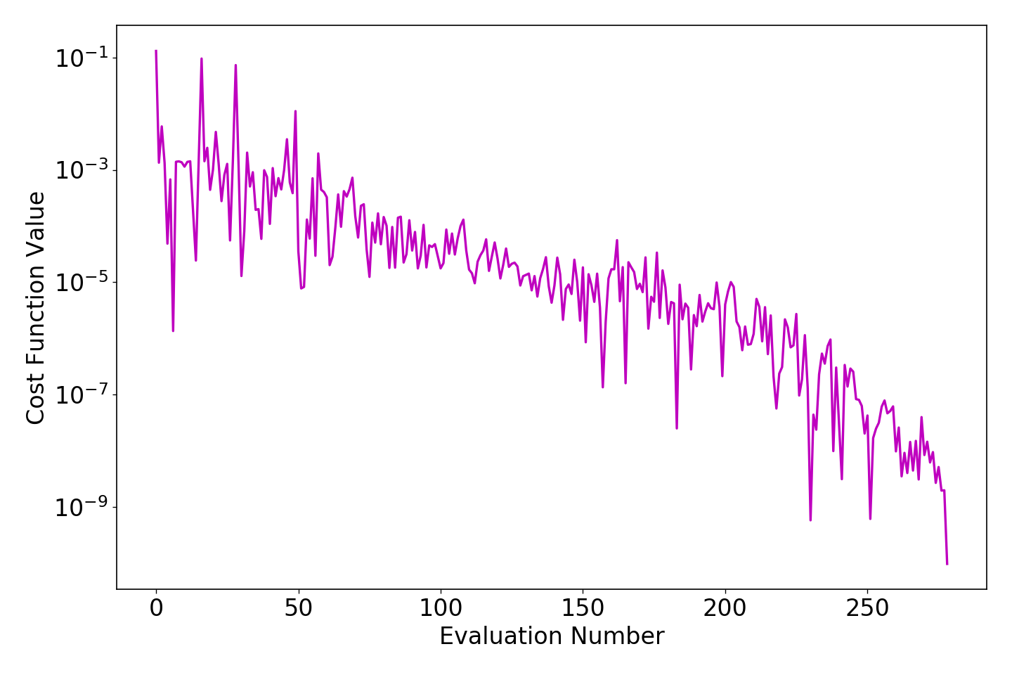
The path opt/trainingset_best_params always stores the best parameters on disk. The opt/*history.dat contains all parameter vectors sampled during the optimization and the respective fitness function value. We can plot the history by typing
>>> params plot trainingset_history.dat
Saved plot to './trainingset_history.png'
in a terminal after changing to the opt directory. The resulting image will be a plot of the evaluation number against the fitness function value and will look similar to this:
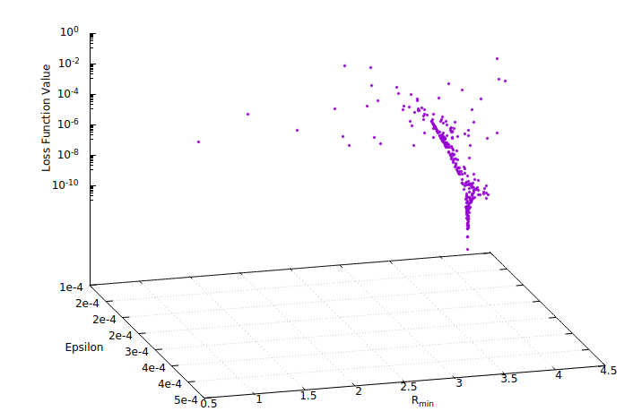
Note
Because the LJ Engine only has two parameters (Epsilon and R_min), we can visualize the whole search space. If gnuplot is installed on your system, you can use the following script to generate an interactive 2d plot:
set logscale z
set xl "Epsilon"
set yl "R_{min}"
set zl "Loss Function Value" rotate by 90
set format x "%.0te%L"
set format z "10^{%L}"
set grid
splot 'trainingset_history.dat' u 3:4:2 pt 7 ps .4
pause -1
The resulting figure should look similar to:
The data folder contains other useful information about the optimization, which is further subdivided into contributions, and residuals. Contributions include data files that print the residuals vector \((w/\sigma)(y-\hat{y})\) per data set each time an improved parameter set is found. The name of each data file is constructed from the evaluation number and the respective loss function value at that evaluation such that the resulting file name is ‘EVALNUM_fx_FXVALUE.dat’.
Important
The generation of all *.dat files does not happen automatically. For this functionality, the Logger callback has to be passed to the Optimization class.
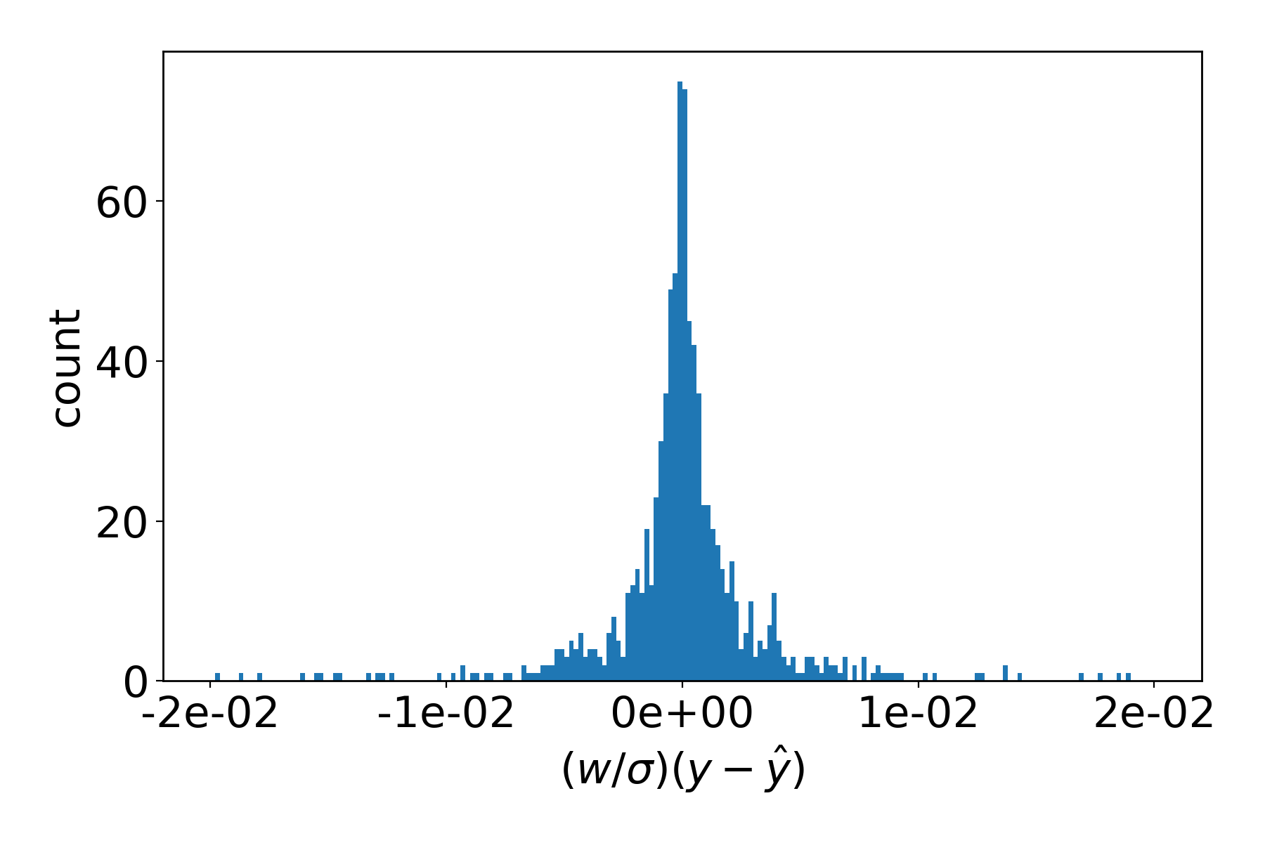
Any of the data files can be plotted. Change directory into data/residuals/trainingset and plot with
>>> params plot 000000_* --xmax 0.02 --bins 200
Saved plot to './000000_fx_XXX.png'
The resulting figure depicts how close the (weighted) atomic forces \(\hat{y}\), as computed with the the initial parameters \(\boldsymbol{x}_0\), are to the reference values \(y\):
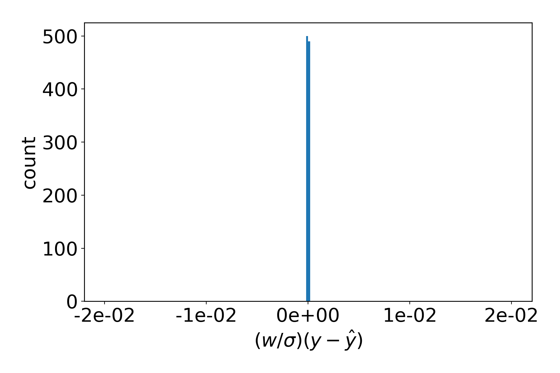
As a contrast, calling params plot --xmax 0.02 --bins 200 without a filename (which is shorthand
for plotting the most recent *.dat file in the directory) will produce the same plot for the last
evaluated parameter set:
Note
You can plot any *.dat file with params plot PATH.
When PATH is a directory, the most recent file will be plotted.
Leaving out the PATH argument will try and plot in the current directory.
For more information about plotting type params plot -h in your
terminal.
The data files in the contributions directory contain contribution of every data set entry to the overall fitness function value.
5.1.3. Modifying the example
The script contains a lot of comments and suggestions on what else can be done at every step.
- Here are a few more:
- Change the reference engine to something other than LJ
- Add more properties to the training set
- Optimize only epsilon / r_min, leaving the other parameter constant