5.2. Parameterization of a Water Force Field with ReaxFF
In this example a ReaxFF force field Water2017.ff will be reparameterized to describe the H–OH bond dissociation energy with with ADF as the reference engine. The workflow script is stored in $AMSHOME/scripting/scm/params/examples/ReaxFF_Water/runme.py, the complete script can also be viewed below.
- The script covers the following steps:
- Conversion of
.bgffile to aJobCollection - Construction of the training set
- Definition an
EngineCollectionand the Reference Engine - Calculation of the reference data
- Parameterization with the
CMAOptimizer - Generation of plots to evaluate the performance of the newly found parameters
- Conversion of
We start by instantiating a training data set, engine collection and limiting the total optimization time to five minutes for the sake of this example:
DS = DataSet()                        # Will store our reference results calculated with ADF
EC = EngineCollection()               # Will store the Settings() for the reference Engine: In this case ADF
callbacks = [Timeout(2*60), Logger()] # Optimize for a total of 5 min. Adjust this if the results are bad and you have time
optimizer = CMAOptimizer(popsize=10, sigma=0.3) # CMA is population-based, meaning it will suggest `popsize` new parameter sets at every iteration.
Note
In a real application the optimization time limit is far from sufficient for a good fit, and might in fact not necessarily yield a better force field than the original. If this happens, try increasing the time limit and running again.
Our training set geometries are stored in $AMSHOME/scripting/scm/params/examples/ReaxFF_Water/xyz/movie.bgf.
AMSMovie supports the export of multiple geometries in this format.
We use geo_to_params() to convert it to
plams.Molecule objects and add each geometry to the Job Collection with the respective task.
We are additionally requesting the gradients through the normal_run_settings keyword:
print('Generating job collection  ...')
# Here we are making use of the `geo_to_params` converter function.
# It automatically detects the geometry and settings stored in a .bgf file
# The task for every molecule will be a Single Point, we are additionally requesting gradients
# for every Geometry by providing the respective plams.Settings (see the documentation of `geo_to_params` for more info).
s = Settings()
s.input.ams.Properties.Gradients = 'True'
s.input.ams.Task = 'SinglePoint'
JC = geo_to_params('xyz/movie.bgf', normal_run_settings=s) # Convert a BGF file to a JobCollection instance, include `grads` in every entry.settings
JC.store('jobcollection.yaml')
print("Job collection stored in 'jobcollection.yaml'.")
Before we can start the optimization, we need to define a training set, i.e. decide which systems and system properties \(P(R)\) we are interested in. This happens in the following block:
print('Generating training set   ...')
for name,entry in JC.items():
    DS.add_entry(f"energy('{name}')", 1.0)
    ## Also possible:
    # DS.add_entry(f"forces('{name}')",  2.5)
    # DS.add_entry(f"charges('{name}')", 1)
    # ...
Now that the training set is defined, we need to provide the reference values
for every entry.
We are making use of the JobCollection.run()
method to calculate all jobs defined in our Job Collection.
By additionally passing the engine_settings argument, we specify the reference engine – in this case ADF:
# The reference engine:
e = Engine() # A EngineCollection takes instances of Engine
e.settings.input.ADF # e.settings is a Settings() instance that needs to be populated
EC.add_entry('ADF_engine01',e)

print('Generating reference data ...')
refresults = JC.run(engine_settings=EC['ADF_engine01'].settings) # Run every entry in JC with engine settings defined in line 25
assert all(r.ok() for r in refresults.values()) # refresults is a dict of {id : AMSResults}
DS.calculate_reference(refresults) # Store the reference results in the training set
DS.store('trainingset.yaml')
print("Training set stored in 'trainingset.yaml'.")
The returned refresults can be treated as regular plams.AMSResults, relevant properties
\(P\) are automatically extracted and added to the training set instance.
After all reference values are provided, the data set is stored.
At this point, the data generated by the reference job calculations is no longer needed and can be
deleted from disk. Reference property values will be available in the trainingset.yaml.
Finally, we select the initial force field that needs optimization, pass the previous instances to the Optimization class and start the fitting process:
ffield = ReaxParams('Water2017.ff') # Interface to the force field format
print(f'Will optimize {len(ffield.active.x)} force field parameters.')
optim = Optimization(JC, DS, ffield, optimizer, callbacks=callbacks)
optim.optimize()
The optimization results are written to a new Water2017.ff.optimized file. Afterwards, a few more jobs are started to generate a comparison plot. Once the script is done, the following files should be of interest:
- Water2017.ff.optimized – The optimized parameters, stored in the ReaxFF force field format
- jobcollection.yml – Job Collection holding the settings and geometries extracted from xyz/movie.bgf
- trainingset.yml – The training set data used for the fit
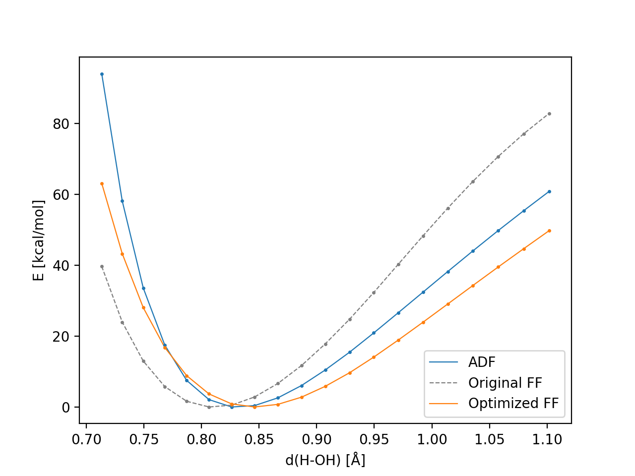
- plot_results.png – Comparison of the dissociation energies for ADF-LDA, Water2017.ff and Water2017.ff.optimized
- plot_optimizer.png – Plot of the best cost function value as a function of the iteration number
The comparison plot plot_results.png should look similar to this:
Execute the script once again to clean up the example folder (deleting all files generated during the optimization).
5.2.1. Complete Example Script
Located in $AMSHOME/scripting/scm/params/examples/ReaxFF_Water/runme.py
#!/usr/bin/env amspython
'''

    Example reparameterization of Water2017.ff with DFT-LDA as the reference engine.
    The training set in xyz/ includes 20 H2O geometries with a different H-OH distance.

'''
import matplotlib as mpl
mpl.use('Agg')
import matplotlib.pyplot as plt
# %matplotlib inline

import numpy as np
import os,sys
from scm.plams import *
from scm.params import *
from scm.params.common.helpers import _cleanup_example_folder as clean
clean(['Water2017.ff.optimized', 'trainingset.yaml', 'opt', 'plot*','plams_workdir', 'jobcollection.yaml'])


totaltime = Timer()

DS = DataSet()                        # Will store our reference results calculated with ADF
EC = EngineCollection()               # Will store the Settings() for the reference Engine: In this case ADF
callbacks = [Timeout(2*60), Logger()] # Optimize for a total of 5 min. Adjust this if the results are bad and you have time
optimizer = CMAOptimizer(popsize=10, sigma=0.3) # CMA is population-based, meaning it will suggest `popsize` new parameter sets at every iteration.


print('Generating job collection  ...')
# Here we are making use of the `geo_to_params` converter function.
# It automatically detects the geometry and settings stored in a .bgf file
# The task for every molecule will be a Single Point, we are additionally requesting gradients
# for every Geometry by providing the respective plams.Settings (see the documentation of `geo_to_params` for more info).
s = Settings()
s.input.ams.Properties.Gradients = 'True'
s.input.ams.Task = 'SinglePoint'
JC = geo_to_params('xyz/movie.bgf', normal_run_settings=s) # Convert a BGF file to a JobCollection instance, include `grads` in every entry.settings
JC.store('jobcollection.yaml')
print("Job collection stored in 'jobcollection.yaml'.")


print('Generating training set   ...')
for name,entry in JC.items():
    DS.add_entry(f"energy('{name}')", 1.0)
    ## Also possible:
    # DS.add_entry(f"forces('{name}')",  2.5)
    # DS.add_entry(f"charges('{name}')", 1)
    # ...


# The reference engine:
e = Engine() # A EngineCollection takes instances of Engine
e.settings.input.ADF # e.settings is a Settings() instance that needs to be populated
EC.add_entry('ADF_engine01',e)

print('Generating reference data ...')
refresults = JC.run(engine_settings=EC['ADF_engine01'].settings) # Run every entry in JC with engine settings defined in line 25
assert all(r.ok() for r in refresults.values()) # refresults is a dict of {id : AMSResults}
DS.calculate_reference(refresults) # Store the reference results in the training set
DS.store('trainingset.yaml')
print("Training set stored in 'trainingset.yaml'.")


ffield = ReaxParams('Water2017.ff') # Interface to the force field format
print(f'Will optimize {len(ffield.active.x)} force field parameters.')
optim = Optimization(JC, DS, ffield, optimizer, callbacks=callbacks)
optim.optimize()


ffield.write('Water2017.ff.optimized') # and write the optimized ffield to 'Water2017.ff.optimized'
print('\n=== === ===')
print(f'Done after {totaltime()}.')
print(f'Running the script again will clean up the directory.')
print('=== === ===\n')
5.2.2. Changing the Example Script
Based on the original script above, the user could try the following, in order to familiarize oneself with the ParAMS package:
- Add more structures to the job collection
- Fit other properties in addition to energies
- Experiment with different CMA settings, especially
sigmaandpopsize. - Use a different reference engine
- Add external reference values to the training set, instead of calculating them