Core Ionization Potentials (XPS) of thiophene

This tutorial demonstrates how to calculate core Ionization Energies (IE) as probed in X-ray Photoemission Spectroscopy (XPS). After calculating the IEs of a thiophene molecule, one can assign the experimental XPS peaks nicely to the different carbon sites in the molecule. The tutorial is based on the publication C. Grazioli, O. Baseggio, M. Stener, G. Fronzoni, M. de Simone, M. Coreno, A. Guarnaccio, A. Santagata, and M. D’Auria, Study of the electronic structure of short chain oligothiophenes, J. Chem. Phys. 146, 054303 (2017). .

Preparation

Before the computation of IEs, the molecular structure of interest should be optimized.

Note

The geometry used in this tutorial has been relaxed with a BP86/TZP DFT calculation.

Setup

Begin by importing the coordinates and setting up the general parameters for the DFT calculation

1. Download the coordinates thiophene.xyz and import them into AMSinput

2. Switch to the and select Task → Single Point

3. Check the Unrestricted checkbox

4. Select XC Functional → GGA → BP86

5. Select Basis set → TZP

6. Select Frozen core → small

Remark: an unrestricted calculation is not needed for a closed shell molecule, but in this case it is handy, since later we will read the electron configuration of this calculation and change it to an open shell electron configuration.

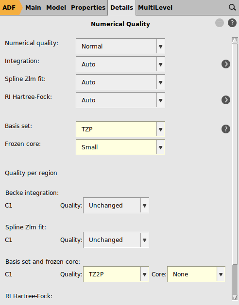
Next, assign a region to one carbon atom to allow specifying a larger all electron basis set to that atom. The trick used here is that a frozen core basis set is used on all atoms except the carbon atom of interest, such that later one can remove 1 electron from the 1s orbital on this carbon atom, without the risk that during the SCF this core hole becomes nonlocal, since all other carbon 1s orbitals are in the frozen core.

1. Switch to the Model → Regions panel

2. Select one of the Carbon atoms next to the Sulfur

3. Click on the

4. Name the region C1

to define a large basis set for this Carbon atom only:

1. Switch to the panel Details → Numerical Quality

2. At the bottom, select Quality → TZ2P and Core → None for the C1 region.

3. Save and Run the calculation.

Results

Once the calculation is finished, open the output (or logfile) and note the bonding energy.

Finally, create a hole state and calculate the bonding energy

1. In AMSinput, switch to the panel Model → Spin and Occupation

2. Change the occupation of the lowest beta orbital to 0

3. Save and Run

Again, the bonding energy is reported in the output file (or logfile) once the calculation has finished. The energy difference between the two bonding energies equals the core Ionization Potential (IP):

\[IP(\textrm{C1,1s}) = E_{hole} - E = 237.5602 -(-53.0143) = 290.5745 \textrm{ eV [Exp.:290.60 eV]}\]

Repeating the calculation with one of the Carbon atoms opposite the Sulfur atoms yields the second IP:

\[IP(\textrm{C2,1s}) = E_{hole} - E = 237.2850 -(-53.0131) = 290.2981 \textrm{ eV [Exp.:290.35 eV]}\]

The computed IPs agree very well (probably due to error cancellation) with the fitted experimental values published in 1. Note that typically one is more interested in the difference of the IPs at different carbon atoms (chemical shifts in carbon 1s IP). Here the calculated difference is 0.28 eV, which is close to the experimental value of 0.25 eV.

1

C. Grazioli1, O. Baseggio, M. Stener, G. Fronzoni, M. de Simone, M. Coreno, A. Guarnaccio, A. Santagata, and M. D’Auria Study of the electronic structure of short chain oligothiophenes, J. Chem. Phys. 146, 054303 (2017)