QM/FQ coupled to MD sampling¶

Test case: UV-Vis spectrum of Methyloxirane (MOX) in aqueous solution¶

In this tutorial, we will simulate the UV-vis absorption spectrum of 2-Methyloxirane in water using the QM/FQ method. Being a polarizable QM/MM model, it is composed of two major steps: (1) the solute-solvent configurational space must be sampled based on a molecular dynamics (MD) simulation, and then (2) the spectrum is evaluated via a number of QM/FQ calculations performed on a set of snapshots extracted from the MD. Both the correct sampling of the configurational space and the subsequent QM calculations upon the solvated molecules are crucial to the quality of the end results.

For more information on the proper way to simulate spectroscopic properties of molecules in aqueous solution see: (1) T. Giovanni et al, “Molecular spectroscopy of aqueous solutions: a theoretical perspective” Chem. Soc. Rev. 49 (2020) 5664.

For more details on the QM/FQ models and its proper use, please see: (2) T. Giovannini et al, “Theory and algorithms for chiroptical properties and spectroscopies of aqueous systems” Phys. Chem. Chem. Phys. 22 (2020) 22864, (3) C. Cappelli, “Integrated QM/polarizable MM/continuum approaches to model chiroptical properties of strongly interacting solute-solvent systems” Int. J. Quantum Chem. 116 (2016) 1532.

The tutorial is divided into two stages: first, we set/run the MD, and then we set/run the QM/FQ calculations. Furthermore, we have two routes:

Route # 1: Written for standard AMS users. Both MD (in AMS) and QM/FQ simulations are explained.

Route # 2: Written for those who already run the MD simulation either in AMS suite or in another package like GROMACS, AMBER, etc, as long as they have any snapshot. This route starts in Step 4, item b, where the QM/FQ simulations are outlined.

Route # 1 (AMS users)

For this simulation, we will use the Force Field engine through the AMS driver program. We suggest read the AMS Molecular Dynamics documentation to get familiar with the details about Molecular Dynamics simulations in the AMS suite.

To start AMSjobs on a Unix-like system, enter the following command:

cd

amsjobs &

On Windows, one can start AMSjobs by double-clicking on the AMS-GUI icon on the Desktop:

Double click the AMS-GUI icon on the Desktop

On Macintosh, use the AMS2021.xxx program to start AMSjobs:

Double click on the AMS2021.xxx icon

You can make a directory for the tutorial by selecting the File → New Director command, typing the directory name, and Return. Change into that directory by clicking once on the folder icon in front of it.

Step 1: Building the system¶

a) Drawing the solute¶

The first thing you need to do is create the solute, in this case, a 2-Methyloxirane molecule. You could build it yourself in AMSinput for a molecule inside AMSinput, or just import it from any database. The steps are as follows:

Start AMSinput via SCM → New Input
Select the atoms-tool, add hydrogens, edit bonds, etc. You can also click into the search box () and type “methyloxirane” and select 2-methyloxirane (ADF) from the drop-down menu. The ‘(ADF)’ string in the search results means that the molecule has already been optimized by ADF, using the BP86 XC potential with a TZP basis set and small core.
If you build your own structure, you can pre-optimize it by clicking on 

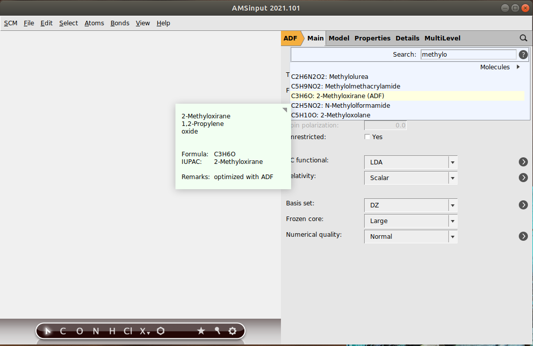
After loading or drawing the structure, you will see it in the drawing area of the molecule editor (the dark area on the middle left side). Click somewhere in the drawing area to deselect all the atoms.

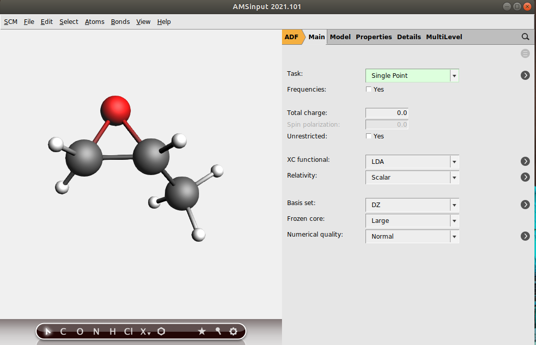
You can rotate, translate, and zoom your molecule using the mouse.

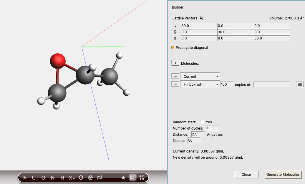
b) Creating the box¶

Now you have to put the solute inside a box, change the third dimension of the lattice vectors, and adjust them depending on the size of the solute and the kind of box you are interested in. To do that,

1. Open the builder tool by clicking: Edit → Builder

2. Make a box of 30x30x30 Angstrom by typing 30 into the diagonal elements of the Lattice vectors.

For larger solvated molecules it is recommended to use a larger box.

c) Adding the solvent¶

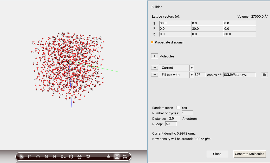
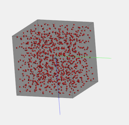
By using the Builder tool in AMSinput, you can easily fill the box with solvent molecules, water for this case, and know the density of the entire system after the water has been added. Again in the Builder panel:

Type ‘water’ in the line with ‘Fill box with’, in the field after copies of:
Select Water (ADF) from the search results
Specify 897 copies. Check the predicted density: 0.9972 g/mL
Click the Generate Molecules button on the bottom

Notice that the solvent molecules are generated at random positions and orientations, with the constraint that all atoms (between different molecules) are at least the specified distance (2.5 Angstrom) apart.

Close the Builder tool by clicking the Close button
Select Force Field engine by switching to the Force Field panel:   → 
Set Periodicity → Bulk. It means 3-dimensions
Click View → Periodic → Show Unit Cell to visualize the box
Rotate to your favorite view

Turn on/off periodic view: View → Periodic → Periodic View or use the bottom to activate/deactivate the periodic view tool.

Step 2: MD equilibration¶

In this tutorial, we start with a short preparation/equilibration run.

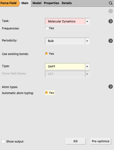
On the right side of the AMSinput window, we already have selected the :

Select Task → Molecular Dynamics
Select Type → GAFF and set the Force Field to be used in the non-reactive MD. UFF, Amber95, Tripos5.2, and a User-Defined Force Field are other possible choices.
Enable Automatic atom typing, which will use the Antechamber program to automatically determine the atom types for the GAFF Force Field

a) Configuring the duration and temperature of the equilibration trajectory¶

Click on  next Task → Molecular Dynamics to go to the Model → MD panel
Configure 100000 steps with a time step of 0.5 fs (Click on a unit to change the unit, your choice will be remembered). This will result in a 0.05 ns (50 ps) long trajectory.
Set the sampling frequency to 100. With a total of 100000 steps, this will result in 1000 recorded samples.
Set the Initial temperature to 300K.
Set Initial velocities to Random

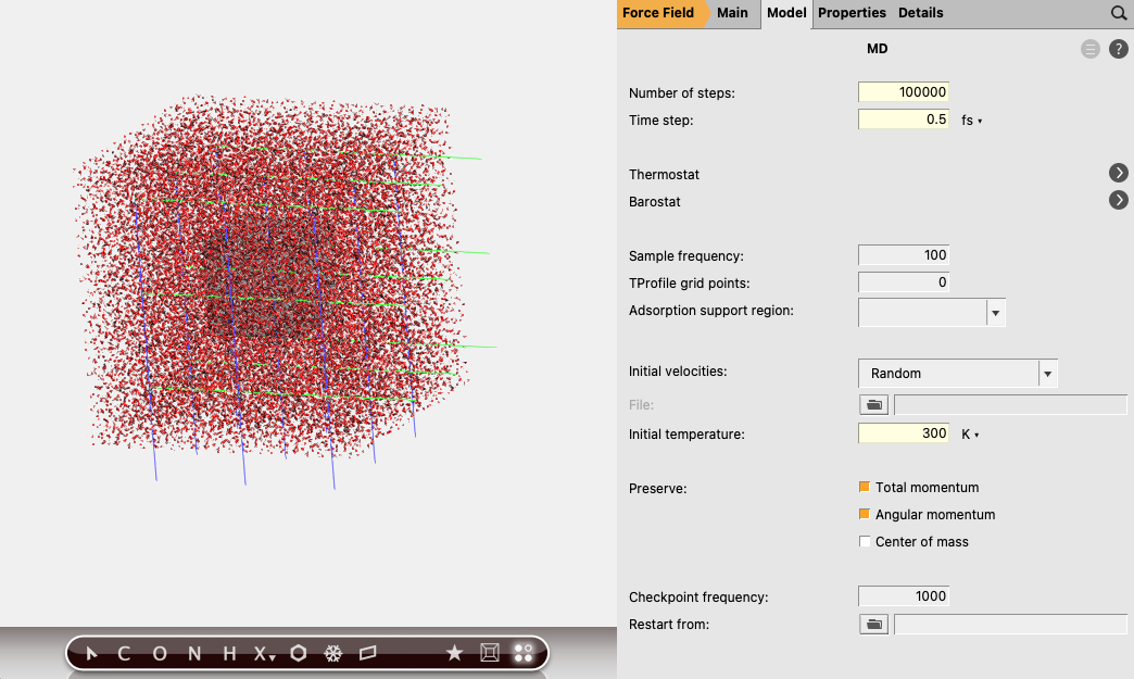
The time step should not be set larger than 0.5 fs because of OH and CH bonds. In an MD run with fixed OH and CH bond lengths one could use a larger time step size, like 2 fs. For some systems one may need a larger number of steps to reach equilibrium, but that is not needed in this case.

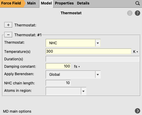
b) Defining the thermostat for equilibration¶

You have set an initial temperature of 300 K, but to maintain this temperature throughout the simulation it is also necessary to attach a thermostat to the system. In the equilibration step the Berendsen thermostat will be used.

Click on  next to the Thermostat to go to the Model → Thermostat panel
Click the  button to add a thermostat to the simulation
Select Thermostat → Berendsen, which can be used for equilibration
(note that NHC (Nosé–Hoover chain) is the preferred thermostat for production runs)
Set 300 K as the Temperature
Set 100 fs as the damping constant. Click on a unit to change the unit

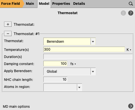
It is also possible to start with a low-temperature MD to relax the initial set-up, or to define different temperatures for the components of the system, using several thermostats for different regions. To that end, you first must define two new regions by using the Regions panel, but it is out of the scope of this tutorial, so, for your solvated 2-Methyloxirane, you will use a single thermostat.

6. Click on

next to MD main options

c) Defining the barostat for equilibration¶

Just like using a Thermostat to control the temperature of the system, a Barostat can be applied to keep the pressure constant by adjusting the volume.

Click on  next to Barostat to go to the Model → Barostat panel.
Select Berendsen from the menu Barostat
Set the desired Pressure to 1.0 atm.
Set the Damping constant to 500 fs. Click on a unit to change the unit
Select XYZ from the menu Equal (such that the box stays cubic)

6. Click on

next to MD main options

d) Run the MD for equilibration¶

Now you can run your setup.

Use the File → Run command.
When asked to save your input, save it with a name of your choice. Make sure you select the Tutorial directory that you made
The AMSjobs window comes to the front and your job starts running.

Once your job starts running, AMSjobs will show the progress of the calculation: the last few lines of the logfile:

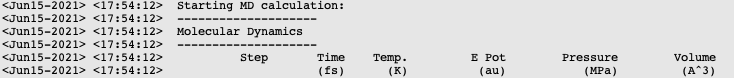
Note that while running, the job status symbol in AMSjobs changes. If you wish to see the full logfile while the calculation is running, just click on the logfile lines in the AMSjobs window, and it will show the logfile in the AMStail window.

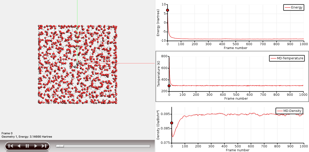
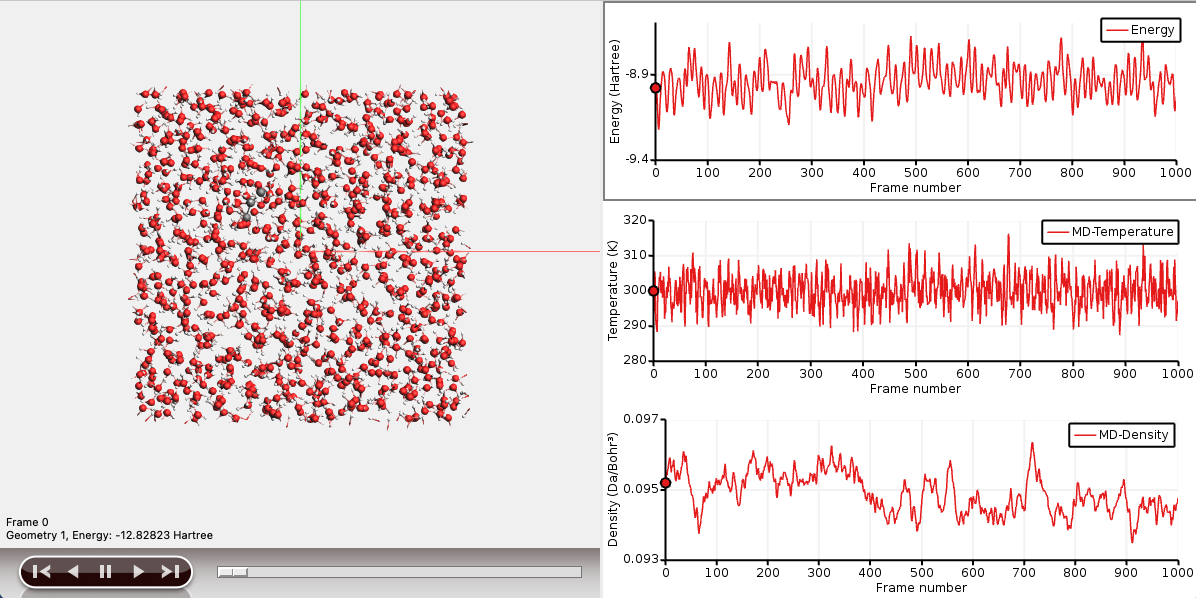
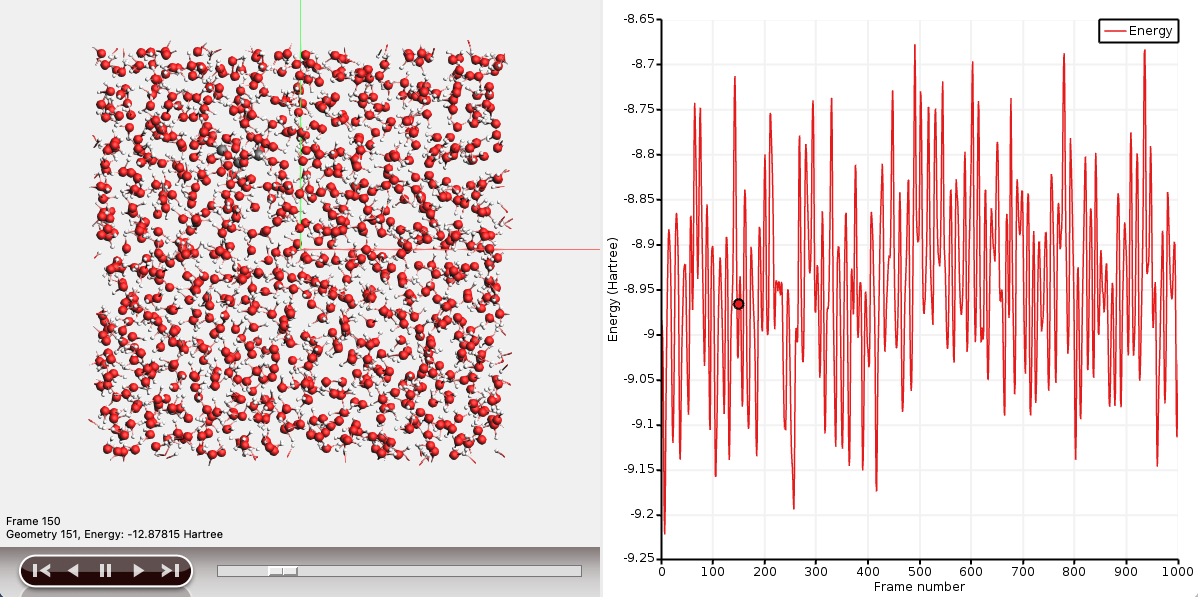
In the calculation first the atom types for the GAFF force field are determined, which will take some time. Next the MD steps are calculated. Let the calculation run for at least half an hour. While it is running, you can already follow its progress in AMSmovie.

4. In the AMSInput window, click SCM → Movie

The graph on the right-hand side shows the energy as a function of the trajectory step.

You can explore different MD properties along the trajectory when it is ready or even if the simulation is still running.

Use the Graph → Add Graph menu command

Click MD Properties → Temperature

Now you have two graphs. One of them is the ‘active’ graph. When you make a new graph it will always be the active graph. You can also make a graph active by clicking on it.

You can show several graphs for different properties at the same time. Temperature and Density are useful properties to evaluate the quality and convergence of your MD simulation.

Let the calculation finish. This might take around a few hours, depending on your computer resources.

Wait until AMStail shows ‘Job … has finished’ as the last line

In the dialog that pops up, Select the ‘Use MD velocities for AMS MD restart’ checkbox

click ‘Yes, new job’ to update the coordinates and make a new job

Step 3: MD production simulation¶

Here we will set up the production stage of the MD. This MD run uses the results of the equilibration run. Most setting are the same as in the equilibration run, except the settings for the thermostat. In this production run in this tutorial we will also use 100000 steps with a time step of 0.5 fs.

a) Defining the thermostat of the production run¶

1. Go to the Model → Thermostat panel

2. Select Thermostat → NHC (Nosé–Hoover chain), the preferred thermostat for production runs

b) Run the MD production simulation¶

Now you can run your setup.

Use the File → Run command.
When asked to save your input, save it with a name of your choice. Make sure you select the Tutorial directory that you made
The AMSjobs window comes to the front and your job starts running.

Let the calculation run for at least half an hour. While it is running, you can already follow its progress in AMSmovie.

Let the calculation finish. This might take around a few hours, depending on your computer resources.

Wait until AMStail shows ‘Job … has finished’ as the last line

In the dialog that pops up, click ‘Yes’ to update the coordinates

Step 4: Setting up the QM/FQ calculations¶

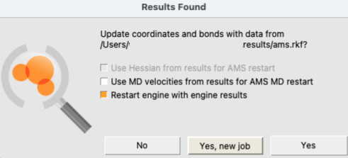
a) Extracting snapshots from the MD runs¶

Once your trajectory is ready, you can open it with AMSMovie and save the geometry for any snapshot.

From the AMSjobs window, select the MD production job and click SCM → Movie
You can select your desired frame by moving the slider through the steps of the trajectory. Use the left and right arrow keys to single-step through the frames.
In AMSmovie, Use the File → Save geometry command
When asked to save your geometry, the suggested filename contains the number of the frame (ams.150.xyz) but you can save it with a name of your choice.
Do this for one more frame.

You can also save the xyz coordinates for the entire trajectory by using File → Export trajectory as → XYZ(.xyz) but in this tutorial, we will use just two of the snapshots.

Now you can close all windows that belong to this tutorial:

Select the SCM → Quit All command in any AMS-GUI window

AMS users should continue with the next Route # 2 to set up the QM/FQ calculations (see below).

Route # 2 (MD-experienced users and AMS users who already run the MD)

MD-experienced users can start the tutorial here if they already have at least two snapshots extracted from any trajectory.

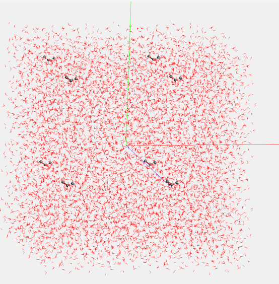
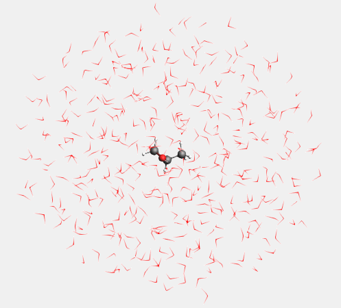
b) Removing PBC and cutting spheres¶

This step is to be carried out if you have not removed periodic conditions yet, or if you have not cut your snapshot yet, or if you want to reduce the size of the sphere. In the AMSjobs window,

Start AMSjobs
Start AMSinput via SCM → New Input
In the AMSinput window,  Select File → Import Coordinates… and select the file containing the data for the snapshot, it can be either a .pdb or a .xyz file extension. For the present case, it will be ‘ams.150.xyz’
Use a supercell if the size of the box is smaller than the size of the solute + 2 times the radius of the cutting sphere + 2 times the size of the solvent. Select Edit → Crystal → Generate Super Cell…
Select one of atoms of a water molecule. Select → Select Molecule. Select → Select Atoms Of Same Type. Select View → Molecule → WireFrame (or Hidden). Only the carbon atoms of the solute should be visible as balls now.
Click at any place to deselect all atoms

Select one of the carbon atoms belonging to (one of) the solute(s).
Select Edit → Set Origin and select Edit → Crystal → Map Atoms To (-0.5..0.5) in order to make this atom the center of the box.
Select ADF engine by switching to the ADF panel:  → 
Select → Select Molecule. Your entire solute molecule should appear selected.
Select → Select within Radius. Write a value for the distance, in Angstroms and Press OK. The radius assures the convergence of the computed data. For small solutes, we suggest cutting 12 Å sphere centered at the solutes’ geometric center, but the choice always depends on the solute size.
Select → Select Molecule. This step is to complete the water molecules placed at the boundaries of the sphere
Select → Invert Selection
Finally, Press backspace key on your keyboard, or go to Atoms → Delete Atoms in the GUI to remove the molecules outside the sphere.

c) Definition of the type of calculation, the different regions of the two-layer scheme, and their boundaries¶

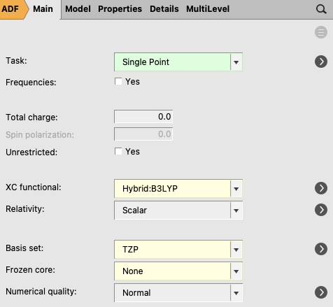
With the sphere already cut, you can proceed with the QM/FQ settings. In this tutorial you will run UV-Vis calculations, thus, in the ‘Main’ space of the panel bar,

Select Task → Single Point
Select XC functional → Hybrid: B3LYP
Select Relativity → Scalar
Select Basis set → TZP and Frozen Core → None
Select Numerical Quality → Normal

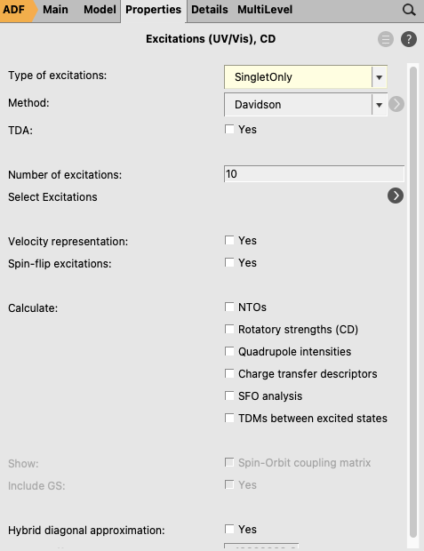
Now, using the panel bar Properties

6. Click on Properties → Excitations (UV/Vis), CD command

7. For the ‘Type of excitations’ option, Select ‘SingletOnly’

Being a QM/MM calculation, we also need to define two regions: one for the solute, and one for the water. To set up these regions:

Click at any place to deselect all atoms
Select the 2-methyloxirane molecule. You can do this by selecting a single atom of this molecule and Select → Molecule
In the panel bar, click the Model → Regions command
Click the   button to add a region
Rename Region_1 to Solute
Select all other atoms of the complex (by Select → Invert Selection)
Click the  button  again, and rename Region_2 to Solvent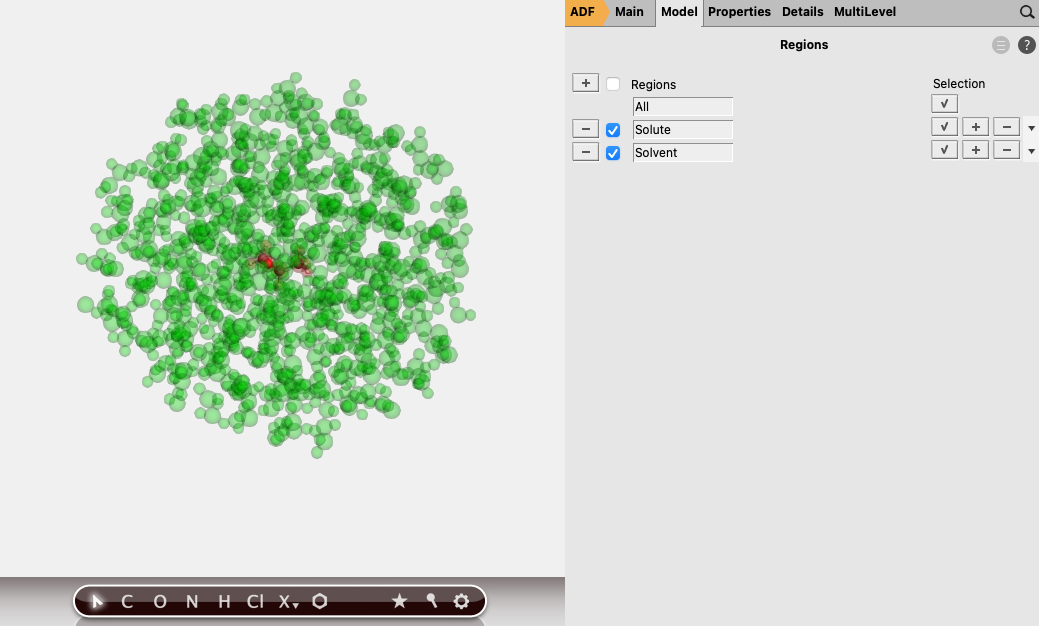
Click on the right arrow at the end of the ‘Solvent’ line. Use the ‘Hidden’ command from the menu that appears. In that way, the molecules in the ‘Solvent’ region are hidden, but the ‘Solvent’ region is still visible because it is colored.

Concerning parametrization, the GUI has parameters for QM/FQ in case water is the solvent in the FQ region.

Use the panel bar Model → QM/FQ command
Check the Enable check button
Click the check button ‘QM part’ for the ‘Solute’ region
Click the check button ‘FQ part’ for the ‘Solvent’ region

The FQ parameters (\(\chi, \eta\)) will appear in the window.

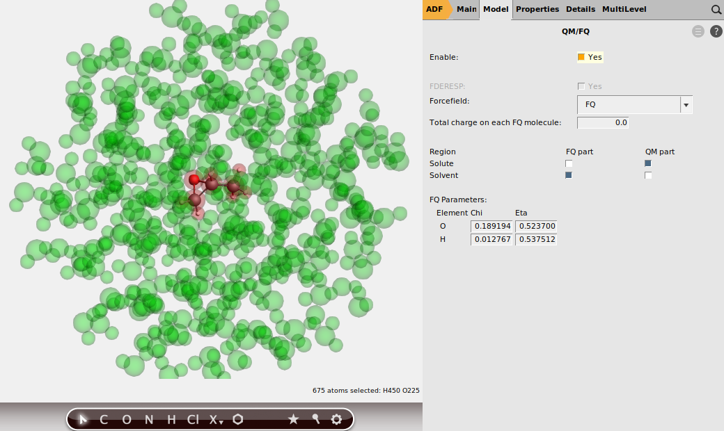
This is all the setup you need. You are now ready to run the QM/FQ calculation

Use the File → Run command.
When asked to save your input, save it with a name of your choice. For example, ‘MOX_QMFQ_frame150’
The AMSjobs window comes to the front and your job starts running.
When asked for a new setup in the dialog that pops up, click ‘No’.

d) Repeat calculation for a different snapshot¶

Follow steps 4b and 4c for a different snapshot. Use a different job name, for example, ‘MOX_QMFQ_frame432’

Step 5: Analyzing the results¶

Once the QM/FQ calculation has finished, the UV-Vis spectrum can be seen from the binary results file.

1. Select SCM → Spectra

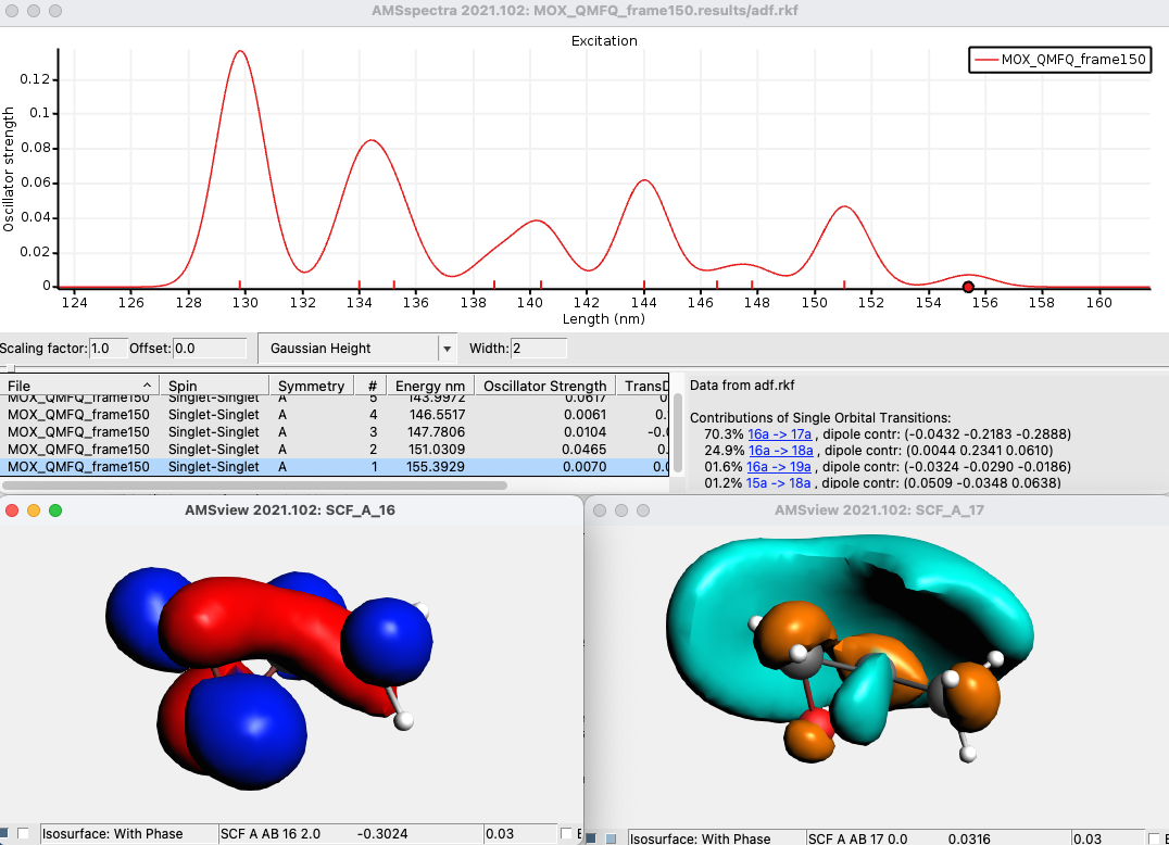
AMSspectra will start and show the calculated absorption spectrum for that specific snapshot. In the window below the spectrum, you will find a table with information. You can get more information by selecting one of the entries (or click on the peak in the spectrum), which will bring some output describing the orbitals involved.

In the table select for example the last Singlet-Singlet peak

The composition of the excitation in terms of molecular orbital transitions is listed on the right side. In many cases, you can visualize relevant orbitals (or also NTOs if you calculated them, note, however, that for hybrids one can only calculate NTOs in case of TDA) with AMSview by clicking on them in the window on the right. The active items are visually marked.

Click on the first major contribution line (with the highlighted orbitals) to bring up 2 pictures of the orbitals, one of the occupied orbital with red and blue lobes and one of the virtual ones with turquoise and ochre lobes.

Close the two windows showing the orbitals.

Next, if you calculated mote than one snapshot.

Select the AMSspectra window
Select File → Add
Navigate to select the result of a different snapshot calculation, for example, MOX_QMFQ_frame432.results/adf.rkf

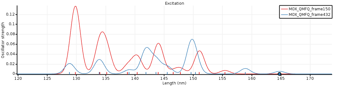
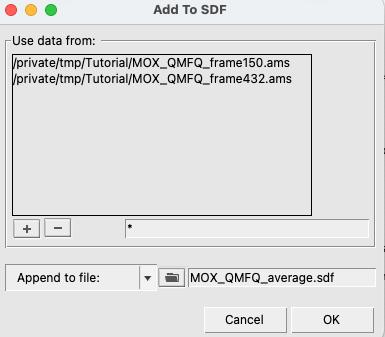
Next an averaged spectrum is calculated.

Select the AMSjobs window
Select the 2 jobs for the calculated snapshots
Select Tools → Add to SDF…
Enter ‘MOX_QM_average.sdf’ for ‘Append to File’
Select ‘OK’

In the AMSjobs window select Job → Refresh List and next select the file ‘MOX_QM_average’
Select SCM → Spectra
Select ‘Uniform’ from the weights pull down underneath the graph (the menu labeled ‘Boltzmann’ at this moment. You may need to increase the size of your AMSspectra window for it to be visible.)
You may want to change the graph title

You can see the individual spectra if one selects View → Average/All Curve. Note that at the moment the excitation spectra are artificially broadened (Width parameter). This broadening can be estimated in a more physical way if one calculates the average spectrum of excitation energies for many MD snapshots.