pyCRS : Basic usage for PropPred and FastSigma
Basic usage
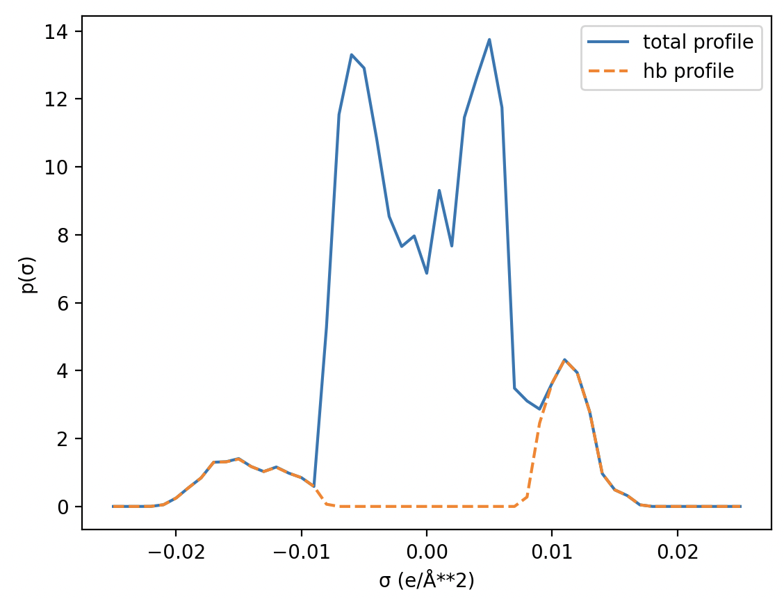
This basic example provides a minimal script input a molecule (paracetamol) as a smiles string, calculate a single property, and then estimate the default (COSMO-RS) sigma profile.
[show/hide code]
import pyCRS
import numpy as np
import matplotlib.pyplot as plt

mol = pyCRS.Input.read_smiles("CC(=O)Nc1ccc(O)cc1")  # paracetamol

print("available properties:", pyCRS.PropPred.available_properties)

pyCRS.PropPred.estimate(mol, "hfusion")
print("hfusion value:", mol.properties["hfusion"], pyCRS.PropPred.units["hfusion"])

pyCRS.FastSigma.estimate(mol, method="COSMO-RS", display=False)

sigma_profiles = mol.get_sigma_profile()
print("Total sigma profile:")
print(sigma_profiles["Total Profile"])
print("H-Bonding:")
print(sigma_profiles["H-Bonding Profile"])

chgden = np.linspace(-0.025, 0.025, 51)
plt.plot(chgden, sigma_profiles["Total Profile"], label="total profile")
plt.plot(chgden, sigma_profiles["H-Bonding Profile"], "--", label="hb profile")
plt.xlabel("σ (e/Å**2)")
plt.ylabel("p(σ)")
plt.legend()
plt.show()
The output produced is the following:
available properties: ['acentricfactor', 'autoignitiontemp', 'boilingpoint', 'critcompress', 'criticalpressure', 'criticaltemp', 'criticalvol', 'density', 'dielectricconstant', 'dipolemoment', 'entropygas', 'entropystd', 'flashpoint', 'gformstd', 'gidealgas', 'hcombust', 'hformstd', 'hfusion', 'hidealgas', 'hsublimation', 'liquidviscosity', 'lowflamlimper', 'meltingpoint', 'molarvol', 'parachor', 'radgyration', 'refractiveindex', 'solubilityparam', 'synacc', 'tpp', 'tpt', 'upflamlimper', 'vaporpressure', 'vdwarea', 'vdwvol']
hfusion value: 28.084352493286133 kJ/mol
Total sigma profile:
[0.0, 0.0, 0.0, 0.002353191375733, 0.050697326660157, 0.24713134765625, 0.5523872375488279, 0.840805053710938, 1.301651000976562, 1.316818237304688, 1.408416748046875, 1.173583984375, 1.027912139892578, 1.160888671875, 0.979301452636719, 0.8482666015625, 0.5888519287109371, 5.276319718325397, 11.539728505193898, 13.300330108724362, 12.906459205297642, 10.834775504652777, 8.539289410607651, 7.653812772468701, 7.964459592741903, 6.8641550757498555, 9.304299127480718, 7.66864582217209, 11.452185796196918, 12.639082653211547, 13.748599090727417, 11.745518829550344, 3.4796992518586065, 3.1053283341103315, 2.864667892456055, 3.6309814453125, 4.3218994140625, 3.9415283203125, 2.786376953125, 0.968017578125, 0.48760986328125, 0.319122314453125, 0.047515869140625, 0.0, 0.0, 0.0, 0.0, 0.0, 0.0, 0.0, 0.0]
H-Bonding:
[0.0, 0.0, 0.0, 0.002353191375733, 0.050697326660157, 0.246719360351562, 0.552310943603516, 0.840805053710938, 1.301651000976562, 1.313278198242188, 1.3948974609375, 1.173583984375, 1.027912139892578, 1.15216064453125, 0.979301452636719, 0.8482666015625, 0.5888519287109371, 0.065513610839843, 0.0, 0.0, 0.0, 0.0, 0.0, 0.0, 0.0, 0.0, 0.0, 0.0, 0.0, 0.0, 0.0, 0.0, 0.0, 0.277877807617188, 2.451416015625, 3.6309814453125, 4.3218994140625, 3.9354248046875, 2.78125, 0.968017578125, 0.48760986328125, 0.319122314453125, 0.047515869140625, 0.0, 0.0, 0.0, 0.0, 0.0, 0.0, 0.0, 0.0]
Temperature-dependent properties
This example calculates the vapor pressure and produces a plot of vapor pressure against temperature.
[show/hide code]
import pyCRS
import matplotlib.pyplot as plt

mol = pyCRS.Input.read_smiles("CCCCCCO")

prop_name = "vaporpressure"
pyCRS.PropPred.estimate(mol, temperatures=[290, 295, 300, 305, 310, 315])
print("Results:", mol.properties_tdep[prop_name])

x, y = mol.get_tdep_values(prop_name)
unit = pyCRS.PropPred.units[prop_name]
plt.plot(x, y, "-o")
plt.ylabel(f"vapor pressure ({unit})")
plt.xlabel("Temperature (K)")
# plt.savefig('./pyCRS_PropPred_Tdep.png')
plt.show()
The output shows the format of the results: (temperature, vapor pressure) pairs
Results: [(290.0, 0.0006316340979498092), (295.0, 0.0009549864170162676), (300.0, 0.0014201952225525484), (305.0, 0.002079200184963613), (310.0, 0.0029991100667307634), (315.0, 0.004265490872465904)]
Finally, the plot produced is the following:
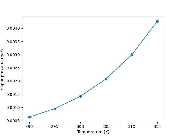
Fig. 4 The estimated vapor pressure versus temperature for 1-Hexanol
Estimating multiple properties
Estimating multiple properties is as simple as supplying a list of property names to the PropPred interface. All properties are estimated by default if no property argument is supplied. In this example, we first estimate a few properties, and then estimate all properties.
[show/hide code]
import pyCRS


def print_props(mol):
    for prop, value in mol.properties.items():
        unit = pyCRS.PropPred.units[prop]
        print(f"{prop:<20s}: {value:.3f} {unit}")

    for prop, value in mol.properties_tdep.items():
        print(f"{prop:<20s}:")
        unit = pyCRS.PropPred.units[prop]
        propunit = f"{prop} ({unit})"
        print("T (K)".rjust(30) + f"{propunit:>30s}")

        for t, v in value:
            print(f"{t:>30.3f}{v:>30.8g}")


mol = pyCRS.Input.read_smiles("CCCCCCO")

props = ["meltingpoint", "boilingpoint", "density", "flashpoint", "vaporpressure"]
pyCRS.PropPred.estimate(mol, props, temperatures=[298.15, 308.15, 318.15, 328.15])
print("Results (temp-independent) :", mol.properties)
print("Results (temp-dependent)   :", mol.properties_tdep)

# we can also estimate all properties by supplying the property name 'all' or simply omitting this argument
pyCRS.PropPred.estimate(mol, temperatures=[298.15, 308.15, 318.15, 328.15])
print_props(mol)
The output produced is the following:
Results (temp-independent) : {'boilingpoint': 435.7771752780941, 'density': 0.7918196941677842, 'flashpoint': 342.2705857793571, 'meltingpoint': 231.1412353515625, 'molarvol': 0.1289491355419159}
Results (temp-dependent)   : {'vaporpressure': [(298.1499938964844, 0.00122854727137622), (308.1499938964844, 0.0026233569814824815), (318.1499938964844, 0.005288582928457778), (328.1499938964844, 0.010122673317257832)]}
boilingpoint        : 435.777 K
criticalpressure    : 34.349 bar
criticaltemp        : 878.101 K
criticalvol         : 0.404 L/mol
density             : 0.792 kg/L (298.15 K)
dielectricconstant  : 10.951
entropygas          : 439.885 J/(mol K)
flashpoint          : 342.271 K
gidealgas           : -131.869 kJ/mol
hcombust            : -3678.121 kJ/mol
hformstd            : -384.388 kJ/mol
hfusion             : 18.505 kJ/mol
hidealgas           : -316.821 kJ/mol
hsublimation        : 80.980 kJ/mol
meltingpoint        : 231.141 K
molarvol            : 0.129 L/mol
parachor            : 289.059
solubilityparam     : 10.129 √(cal/cm^3)
synacc              : 6.747
tpt                 : 230.404 K
vdwarea             : 171.059 Ų
vdwvol              : 120.519 ų
liquidviscosity     :
                         T (K)        liquidviscosity (Pa-s)
                       298.150                  0.0044653385
                       308.150                   0.003363708
                       318.150                  0.0025843814
                       328.150                  0.0020210327
vaporpressure       :
                         T (K)           vaporpressure (bar)
                       298.150                  0.0012285473
                       308.150                   0.002623357
                       318.150                  0.0052885829
                       328.150                   0.010122673
Calculating sigma profiles with all models
This example demonstrates how to calculate COSMO-RS sigma profiles with both available models (SG1 and FS1). We’ll use 4-Methylphenol for this example. The variable ref_sp in the script is the \(\sigma\)-profile calculated in the AMS COSMO-RS.
[show/hide code]
import pyCRS
import matplotlib.pyplot as plt
from pyCRS.Database import COSKFDatabase
from pyCRS.CRSManager import CRSSystem

db = COSKFDatabase("my_coskf_db.db")
db.add_compound("4-Methylphenol.coskf")

cal = CRSSystem()
mixture = {"4-Methylphenol": 1.0}

cal.add_Mixture(mixture, problem_type="PURESIGMAPROFILE")
cal.runCRSJob()
out = cal.outputs[0]
res = out.get_results()

chdens = res["chdval"][0]
ref_sp = res["profil"][0]

# chdens = [-0.025 + 0.001 * x for x in range(51)]
# ref_sp = [0.0, 0.0, 0.0, 0.0, 0.0, 0.170502089, 0.735172882, 0.983838864, 0.86397332, 1.15571158, 0.670512863, 0.793806705, 0.714228251, 0.688547843, 0.72126747, 0.724141667, 0.832938008, 2.33617486, 5.42197092, 8.58230745, 9.84294559, 8.81993395, 8.8093211, 6.79578176, 6.57764296, 6.0780249, 9.19651976, 11.0472172, 12.8025552, 11.1767254, 12.2878801, 10.7212122, 2.77829981, 1.11136819, 1.58235813, 1.13444125, 1.8131698, 2.4446856, 2.02558727, 0.0124393296, 0.0, 0.0, 0.0, 0.0, 0.0, 0.0, 0.0, 0.0, 0.0, 0.0, 0.0]

mol = pyCRS.Input.read_smiles("Cc1ccc(O)cc1")

pyCRS.FastSigma.estimate(mol, method="COSMO-RS", model="FS1")
sp_fs1 = mol.get_sigma_profile()["Total Profile"]

pyCRS.FastSigma.estimate(mol, method="COSMO-RS", model="SG1")
sp_sg1 = mol.get_sigma_profile()["Total Profile"]

plt.plot(chdens, ref_sp, "--", label="Reference $\sigma$-profile")
plt.plot(chdens, sp_fs1, label="FS1 $\sigma$-profile")
plt.plot(chdens, sp_sg1, label="SG1 $\sigma$-profile")
plt.ylabel("Area ($\AA^2$)")
plt.xlabel("$\sigma$")
plt.grid()
plt.legend()
# plt.savefig('./pyCRS_PropPred_SigmaProfile.png')
plt.show()
Finally, the plot produced shows the various \(\sigma\)-profiles produced.
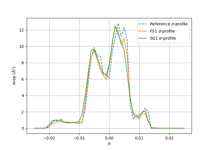
Fig. 5 The sigma profile of 4-Methylphenol