Reparametrizing ReaxFF with the CMA-ES optimizer
Important
This tutorial uses the old standalone ReaxFF program. From AMS2022, we recommend that you instead follow the ParAMS tutorials.
Overview of the workflow
This advanced ReaxFF tutorial will demonstrate how to fit ReaxFF parameters to create a new force field.

The reparametrization workflow consists of the following steps:
Fit a new force field to the reference data
Cross-validate the new force field
If needed: refine training set (add entries, adjust weights…) and re-fit, cross-validate,…
The force field optimization algorithm requires the evaluation of an objective function (aka cost function). For ReaxFF the objective function takes the form:
where the sum runs over all training set entries. Each difference between the reference property (xi,ref) and the ReaxFF value - calculated with your new force field - (xi,ReaxFF) is weighted individually via the weightings σi. The weightings, σi, can be set automatically but will most likely need to be refined manually during the fitting process.
Once the objective function has been set up, the CMA-ES optimizer can be used to fit a set of new parameters. Since the force field optimizers included in AMS, MCFF <MCFFOptimizer> and CMA-ES <cmaes>, are stochastic optimization algorithms, it is advised to run them multiple times, possibly starting from different/random starting conditions. The force fields with the lowest overall value of the objective function can then be tested in a cross-validation scheme.
It’s advised to validate a newly fitted force field by testing it on a set of references that were not used during the training of the force field. This serves as a simple measure against overfitting and provides some direct information on the transferability of the new parameters.
The tutorial is inspired by the work done by A. Vashisth and coworkers on re-fitting an existing ReaxFF force field for usage with the novel bond boost acceleration method :
Like in the paper, the parameters related to C-O, C-N and N-H in the force field CHON-2017_weak.ff are going to be refitted. Both the initial force field and the refitted force field from the paper (CHON-2017_weak_bb.ff) are shipped with AMS2019, so you can compare both with the force field you are going to create in this tutorial.
Assigning weights
Some remarks on weights
The force field optimization algorithm requires the evaluation of an objective function. For ReaxFF the objective function takes the form:
where the sum runs over all training set entries. Each difference between the reference property (xi,ref) and the ReaxFF value - calculated with your new force field - (xi,ReaxFF) is weighted individually via the weightings σi. The weightings, σi, can be set automatically but will most likely need to be refined manually during the fitting process.
If you look at the weights in the above function more closely, you might spot that they can be interpreted in terms of an accuracy or rather a desired accuracy as you don’t know beforehand which accuracy the fitting process will yield in the end. When coming up with weights this view can guide your initial guesses. However, it should also be kept in mind that the relative values of the weights are important too as discussed in the below example.
Let’s assume you have a medium sized organic molecule and you assign a weight of 0.01 to all C-H and all C-O bonds. This scheme will probably not result in a very high accuracy of the C-O bond energies. Why? Simply because there will be much, much more C-H bonds in the system than C-O bonds. Since all errors are going to be summed up, even small changes in the C-H bond energies will affect the value of the objective function more than a medium change in the C-O bond. The optimizer “sees” only a single number, so it’s important to make sure that the objective function is balanced (hence the usage of the terms weight) - or - if it’s biased, it should be biased towards the entries you consider important for your system.
If this left you puzzled, why not take a look at the weights that were used in the published Co trainingset to gain some further inspiration?
How to run the optimizer
At the time of writing there exists no GUI support for the CMA-ES optimizer, instead we use the command line to execute the calculations. If you are unfamiliar with using the command line with AMS, then take a look at the Getting Started page of the scripting docs.
Inside the folder CMA-ES-FIT are three subdirectories, called error_function, input and random_initials as well as a shell script, runner, to start the optimization. Before the script can be used, it has to be declared executable:
chmod +x runner
When run, the shell script will execute the following workflow
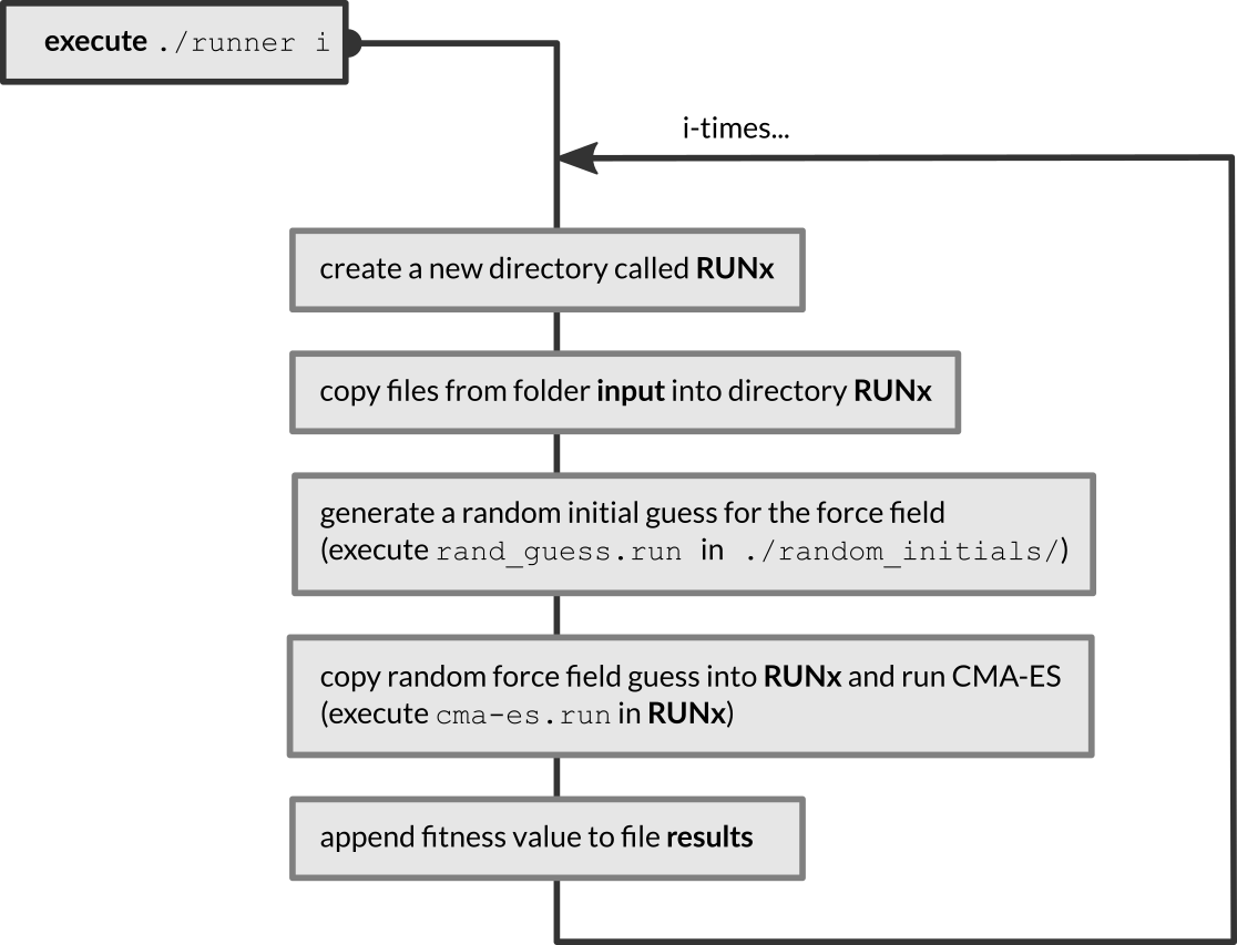
The fitness values of the force fields are appended to the results file, located in the same folder as the runner script. The fitted force fields are found in ./RUNx/ffield_best.
To execute the runner script, provide the number of cma-es runs as an argument. For example, if you want to run 5 CMA-ES runs:
./runner 5
Per default, the optimizations start from a random initial force field. In case you have a reason to believe that your current force field is already a good starting point, it can make sense to not start from a random guess, but start the CMA-ES optimizations from the force field located in training_data/ffield instead. This can be easily done:
./runner 5 norand
Before starting the optimization process the following files need to be present:
File |
Description |
In folder |
|---|---|---|
trainset.in, geo |
The training set. As exported by AMStrain. |
training_data |
trainset.in, geo |
The validation set. As exported by AMStrain. |
error_function |
ffield |
A ReaxFF force field file. Serves as initial guess. |
training_data |
params |
Defines ranges and active parameters during optimization. |
training_data |
For the course of this tutorial you can leave the params and ffield file untouched.
How to monitor a running optimization
A running CMA-ES calculation can be monitored from a second command line window by executing the command:
opt_convergence
inside the folder where a CMA-ES calculation is running. This will print a list of fitness values as function of the iteration index to the screen and create a file called errors.csv at the same time. The fitness values should decrease with increasing number of iterations.
To visualize the convergence, you can call the AMSgraphs module from the command line:
amsgraphs errors.csv
The CMA-ES run typically reaches somewhat asymptotic behavior within just a couple of thousand steps.
How to change optimizer settings
The settings for the CMA-ES optimizer are documented in the CMA-ES manual <cmaes> In the current setup the control file is created by executing the script cma-es.run located in the folder input. The file can be viewed with any editor.
The relevant commands are found at the end of the file. For the CMA-ES optimization these are:
[...snip...]
#CMA-ES settings
5000       mcffit       Max. Number of iterations.
0.00001    ffotol       Convergence criteria.
50         replic       The CMA-ES sample size.
25         mcrxdd       width of the distribution.
                        The smaller this value, the more
                        random (non-local) the search will be.
0          fort99       Do not write fort.99 files

cat > iopt <<eor
7
eor
How to cross-validate a fitted force field
To cross validate a newly fitted force field, supply the path to the force as console argument to the script calculate_errors.run found in the folder error_function. For example, to test the force field fitted in the first CMA-ES run, use the following command (from within the folder error_function):
chmod +x calculate_errors.run
./calculate_errors.run ../RUN1/ffield_best
The result of this calculation is a detailed breakdown of the error function, written to a fort.99 file. Note the root mean square errors reported at the end of the text written to the commandline:
RMSD (Charge):  0.1448 (errors_charge.csv)
RMSD (Bond):    8.5617 (errors_bond.csv)
RMSD (RMSG):   10.9749 (errors_rmsg.csv)
RMSD (Energy): 14.8500 (errors_energy.csv)
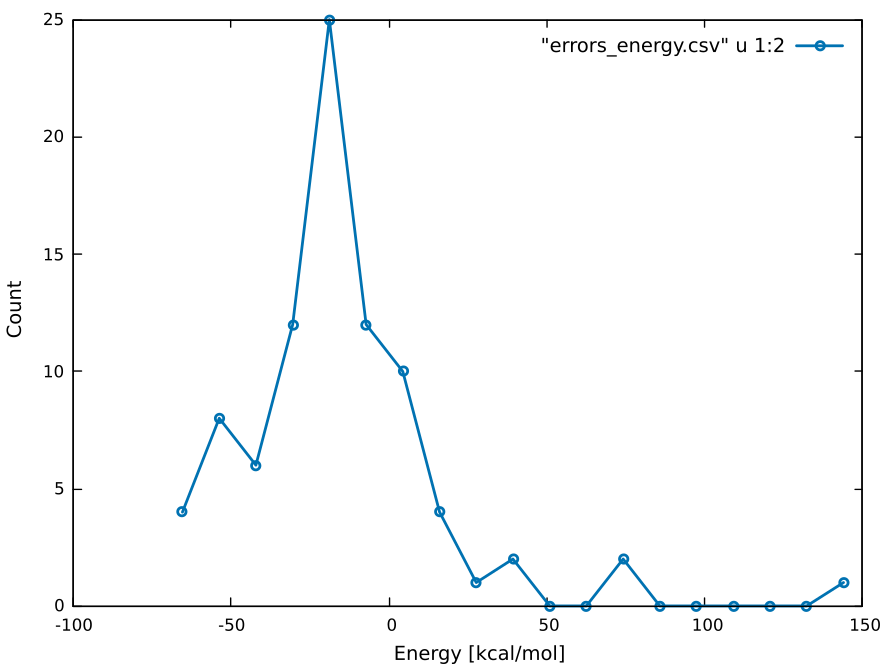
further the differences between predicted and target values are binned and written to error files (filenames are given in parentheses, behind the RMSD) that can be opened with AMSgraphs.
For example:
amsgraphs errors_energies.csv
will show a distribution of the relative error in the energies prediction of your new force field
Running the optimizer
Begin with just two CMA-ES optimization runs, using the default CMA-ES settings:
./runner 2 norand
Note that we are just running two optimizations since the optimization can take a long time, depending ou your hardware and training set. Inside the command line window you can always end a running calculation by pressing CTRL+C. And finally, since we are trying to re-fit an existing force field we can assume the existing ffield is a good starting guess which is why the optimization is run without a random starting guess.
Errors and Cross-validation
Once the calculation has finished, take a look at the results file to find out which optimization run yielded the best fitness value. Keep in mind that the outcome of the optimization runs are non-deterministic and hence your results will differ from the below, but the overall trend should be similar.
For example, a run with 4 independent CMA-ES optimizations, yielded the following results
/home/ole/Workspace/CMA-ES-FIT/RUN1
xbestever found after 1314 evaluations, function value 1.13854e+08
/home/ole/Workspace/CMA-ES-FIT/RUN2
xbestever found after 1116 evaluations, function value 4.77308e+07
/home/ole/Workspace/CMA-ES-FIT/RUN3
xbestever found after 1314 evaluations, function value 5.85587e+07
/home/ole/Workspace/CMA-ES-FIT/RUN4
xbestever found after 1260 evaluations, function value 7.06017e+08
So in this case CMA-ES run #2 yielded the best overall fitness value. Let’s see how well this force field does for the validation test set. From inside the folder error_function run the following command to generate a fort.99 file:
./calculate_errors.run ../RUN2/ffield_best
Next, inspect the resulting RMSD errors:
RMSD (Bond)  :  0.0673 (errors_bond.csv)
RMSD (angle) :  3.4729 (errors_angle.csv)
RMSD (RMSG)  : 33.6747 (errors_rmsg.csv)
RMSD (Energy): 10.9002 (errors_energy.csv)
These errors reflect the weighting in the training set. By assigning a weight of 0.01 to the bond scans in the training data we have put quite some emphasis on the energies and thus it is not surprising that these are reproduced and predicted fairly well. The fit results become even more obvious when comparing with the two force fields CHON2017_weak.ff (our starting guess!) and a refitted version of our starting guess, CHON2017_weak_bb.ff (refitted for usage with the bond boost method).
To calculate the objective function for these force fields, run:
./calculate_errors.run $AMSHOME/atomicdata/ForceFields/ReaxFF/CHON2017_weak.ff
for the force field we used as a starting guess, and
./calculate_errors.run $AMSHOME/atomicdata/ForceFields/ReaxFF/CHON2017_weak_bb.ff
for a force field that was refitted from our starting guess to proper DFT training set. If compare against the refitted force field:
Value in training set |
New FF |
CHON2017_weak_bb.ff |
|---|---|---|
Bonds |
0.0673 |
0.0212 |
Angles |
3.4729 |
1.3347 |
RMSG |
33.6747 |
49.4250 |
Energy |
10.9002 |
26.7171 |
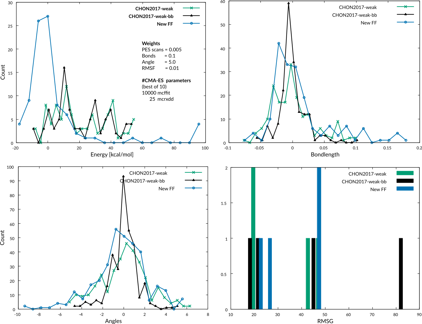
When comparing the error files generated by analysis of the errors you see that the geometries seem to be much better described by the CHON2017_weak_bb.ff. This is due to the fact that we put so much emphasis on the PES scans in our training set.
Refine the training set
Let’s try to adjust the weights in our training data to get better geometries:
Increase the number of steps in the geometry optimizations to 15
Assign a weight of 0.01 to every bond distance in the training.in
Assign a weight of 0.1 to all the energies in trainset.in
and run the CMA-ES optimizer again, followed by a calculation of the objective function for the best force field of this run. The new results should look similar to these finding
Value in training set |
New FF |
CHON2017_weak_bb.ff |
|---|---|---|
Bonds |
0.0275 |
0.0212 |
Angles |
1.7123 |
1.3347 |
RMSG |
28.0047 |
49.4250 |
Energy |
27.4686 |
26.7171 |
The resulting force field is already much closer to the published force field. Again, taking closer look at the error files with AMSgraphs reveals that this weighting scheme seems to result in a much more balanced fore field
Keep in mind that the original force field - of which we have re-used quite some parameters - was fitted against DFT data. In other words, the force field has been trained to reproduce DFT geometries and DFT energies. This means deviations between our DFTB force field and the ‘real’ force fields are to be expected since the comparison isn’t really fair. After all this approach serves for illustrating the concepts and workflow of parameter fitting and not the generation of a production ready force field. If you want to optimize your force field even further, try some of the following:
Training set / Optimization tweaks:
More tests: Apply new force field to MD and geometry optimizations
Try to locate problematic trainset entries and change (decrease) their weights
Increase max. steps for the geometry optimizer
Add more entries
Run more (~10) CMA-ES runs
Check params file in folder input, maybe more parameters need to be fitted?
Check parameter ranges in params file: should a range be increased (compare to your fitted FF)?