Diffusion Coefficient Temperature Dependence
Run Lennard-Jones argon simulations at several temperatures in parallel, extract diffusion coefficients from the mean-squared displacement, and fit an Arrhenius relation to estimate the prefactor and activation barrier.
Diffusion coefficient temperature dependence
The diffusion coefficient often follows an Arrhenius relation with temperature. This example runs Lennard-Jones argon simulations at several temperatures in parallel, extracts the diffusion coefficient from each trajectory, and fits ln(D) versus 1/T to estimate the prefactor and activation barrier.
from scm.plams import Settings


def get_lennard_jones_settings():
    s = Settings()
    s.input.lennardjones.eps = 3.785e-4
    s.input.lennardjones.rmin = 3.81637
    s.input.lennardjones.cutoff = 8.0
    s.runscript.nproc = 1
    return s
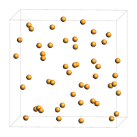
Use a 50-atom argon box and evaluate the diffusion coefficient at 50, 100, 200, and 300 K.
from scm.plams import Molecule, Atom, packmol, preoptimize, view

T_list = [50, 100, 200, 300]
density = 1.0  # g/cm^3
max_correlation_time_fs = 6000
start_time_fit_fs = 3000

Ar = Molecule()
Ar.add_atom(Atom(symbol="Ar", coords=(0, 0, 0)))

mol = packmol(Ar, n_molecules=50, density=density)
mol = preoptimize(mol, settings=get_lennard_jones_settings(), maxiterations=50)
view(mol, height=200, width=200, direction="tilt_z", padding=-2)
If you have multiple cores available, a parallel JobRunner can start the trajectories concurrently.
from scm.plams import config, JobRunner

maxjobs = 4
config.default_jobrunner = JobRunner(parallel=True, maxjobs=maxjobs)
To keep PLAMS from blocking too early, the production jobs use use_prerun=True and the MSD results are only accessed after all jobs have been submitted.
from scm.plams import AMSNVTJob, AMSMSDJob, log

msd_jobs = []
DT_list = []
for T in T_list:
    eq_job = AMSNVTJob(
        name=f"eq_T_{T}",
        settings=get_lennard_jones_settings(),
        molecule=mol,
        temperature=T,
        nsteps=10000,
        samplingfreq=500,
        thermostat="Berendsen",
        tau=100,
        timestep=1.0,
        writebonds=False,
        writecharges=False,
        writemolecules=False,
        writevelocities=False,
    )
    eq_job.run()
    prod_job = AMSNVTJob.restart_from(
        eq_job,
        name=f"prod_T_{T}",
        nsteps=50000,
        samplingfreq=25,
        temperature=T,
        thermostat="NHC",
        use_prerun=True,
    )
    prod_job.run()
    msd_job = AMSMSDJob(
        prod_job, name=f"msd_T_{T}", max_correlation_time_fs=max_correlation_time_fs
    )
    msd_job.run()
    msd_jobs.append(msd_job)


for T, msd_job in zip(T_list, msd_jobs):
    D = msd_job.results.get_diffusion_coefficient(start_time_fit_fs=start_time_fit_fs)
    DT_list.append(D)
    log(f"Temperature {T} K: D = {D:.2e} m^2 s^-1")
[23.03|14:56:29] JOB eq_T_50 STARTED
[23.03|14:56:29] JOB prod_T_50 STARTED
[23.03|14:56:29] JOB msd_T_50 STARTED
[23.03|14:56:29] JOB eq_T_100 STARTED
[23.03|14:56:29] Waiting for job eq_T_50 to finish
[23.03|14:56:29] JOB prod_T_100 STARTED
[23.03|14:56:29] JOB msd_T_100 STARTED
[23.03|14:56:29] JOB eq_T_200 STARTED
[23.03|14:56:29] JOB eq_T_50 RUNNING
[23.03|14:56:29] Waiting for job prod_T_50 to finish
... output trimmed ....
[23.03|14:56:44] JOB msd_T_200 FINISHED
[23.03|14:56:44] JOB msd_T_50 SUCCESSFUL
[23.03|14:56:44] JOB msd_T_100 SUCCESSFUL
[23.03|14:56:44] Temperature 50 K: D = 1.73e-09 m^2 s^-1
[23.03|14:56:44] Temperature 100 K: D = 6.03e-09 m^2 s^-1
[23.03|14:56:44] JOB msd_T_200 SUCCESSFUL
[23.03|14:56:44] JOB msd_T_300 SUCCESSFUL
[23.03|14:56:44] Waiting for job msd_T_200 to finish
[23.03|14:56:44] Temperature 200 K: D = 1.19e-08 m^2 s^-1
[23.03|14:56:44] Temperature 300 K: D = 1.75e-08 m^2 s^-1
import numpy as np
import matplotlib.pyplot as plt
from scm.plams.tools.plot import linear_fit_extrapolate_to_0
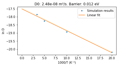
inverted_T_list = 1.0 / np.array(T_list)
ln_D_list = np.log(DT_list)
fit_x, fit_y, slope, intercept = linear_fit_extrapolate_to_0(inverted_T_list, ln_D_list)
D0 = np.exp(intercept)
boltzmann_eV_per_K = 8.617e-5
barrier = -boltzmann_eV_per_K * slope
title = f"D0: {D0:.2e} m²/s. Barrier: {barrier:.3f} eV"
log(title)
fig, ax = plt.subplots(figsize=(6, 3))
ax.plot(inverted_T_list * 1000, ln_D_list, ".", label="Simulation results")
ax.plot(fit_x * 1000, fit_y, label="Linear fit")
ax.set_title(title)
ax.legend()
ax.set_xlabel("1000/T (K⁻¹)")
ax.set_ylabel("ln D")
ax;
[23.03|14:56:44] D0: 2.48e-08 m²/s. Barrier: 0.012 eV
See also
Python Script
#!/usr/bin/env python
# coding: utf-8

# ## Diffusion coefficient temperature dependence
#
# The diffusion coefficient often follows an Arrhenius relation with temperature. This example runs Lennard-Jones argon simulations at several temperatures in parallel, extracts the diffusion coefficient from each trajectory, and fits ``ln(D)`` versus ``1/T`` to estimate the prefactor and activation barrier.
#

from scm.plams import Settings


def get_lennard_jones_settings():
    s = Settings()
    s.input.lennardjones.eps = 3.785e-4
    s.input.lennardjones.rmin = 3.81637
    s.input.lennardjones.cutoff = 8.0
    s.runscript.nproc = 1
    return s


# Use a 50-atom argon box and evaluate the diffusion coefficient at 50, 100, 200, and 300 K.
#

from scm.plams import Molecule, Atom, packmol, preoptimize, view

T_list = [50, 100, 200, 300]
density = 1.0  # g/cm^3
max_correlation_time_fs = 6000
start_time_fit_fs = 3000

Ar = Molecule()
Ar.add_atom(Atom(symbol="Ar", coords=(0, 0, 0)))

mol = packmol(Ar, n_molecules=50, density=density)
mol = preoptimize(mol, settings=get_lennard_jones_settings(), maxiterations=50)
view(mol, height=200, width=200, direction="tilt_z", padding=-2, picture_path="picture1.png")


# If you have multiple cores available, a parallel ``JobRunner`` can start the trajectories concurrently.
#

from scm.plams import config, JobRunner

maxjobs = 4
config.default_jobrunner = JobRunner(parallel=True, maxjobs=maxjobs)


# To keep PLAMS from blocking too early, the production jobs use ``use_prerun=True`` and the MSD results are only accessed after all jobs have been submitted.
#

from scm.plams import AMSNVTJob, AMSMSDJob, log

msd_jobs = []
DT_list = []
for T in T_list:
    eq_job = AMSNVTJob(
        name=f"eq_T_{T}",
        settings=get_lennard_jones_settings(),
        molecule=mol,
        temperature=T,
        nsteps=10000,
        samplingfreq=500,
        thermostat="Berendsen",
        tau=100,
        timestep=1.0,
        writebonds=False,
        writecharges=False,
        writemolecules=False,
        writevelocities=False,
    )
    eq_job.run()
    prod_job = AMSNVTJob.restart_from(
        eq_job,
        name=f"prod_T_{T}",
        nsteps=50000,
        samplingfreq=25,
        temperature=T,
        thermostat="NHC",
        use_prerun=True,
    )
    prod_job.run()
    msd_job = AMSMSDJob(prod_job, name=f"msd_T_{T}", max_correlation_time_fs=max_correlation_time_fs)
    msd_job.run()
    msd_jobs.append(msd_job)


for T, msd_job in zip(T_list, msd_jobs):
    D = msd_job.results.get_diffusion_coefficient(start_time_fit_fs=start_time_fit_fs)
    DT_list.append(D)
    log(f"Temperature {T} K: D = {D:.2e} m^2 s^-1")


import numpy as np
import matplotlib.pyplot as plt
from scm.plams.tools.plot import linear_fit_extrapolate_to_0


inverted_T_list = 1.0 / np.array(T_list)
ln_D_list = np.log(DT_list)
fit_x, fit_y, slope, intercept = linear_fit_extrapolate_to_0(inverted_T_list, ln_D_list)

D0 = np.exp(intercept)
boltzmann_eV_per_K = 8.617e-5
barrier = -boltzmann_eV_per_K * slope
title = f"D0: {D0:.2e} m²/s. Barrier: {barrier:.3f} eV"
log(title)

fig, ax = plt.subplots(figsize=(6, 3))
ax.plot(inverted_T_list * 1000, ln_D_list, ".", label="Simulation results")
ax.plot(fit_x * 1000, fit_y, label="Linear fit")
ax.set_title(title)
ax.legend()
ax.set_xlabel("1000/T (K⁻¹)")
ax.set_ylabel("ln D")
ax
ax.figure.savefig("picture2.png")