Ionic Conductivity¶

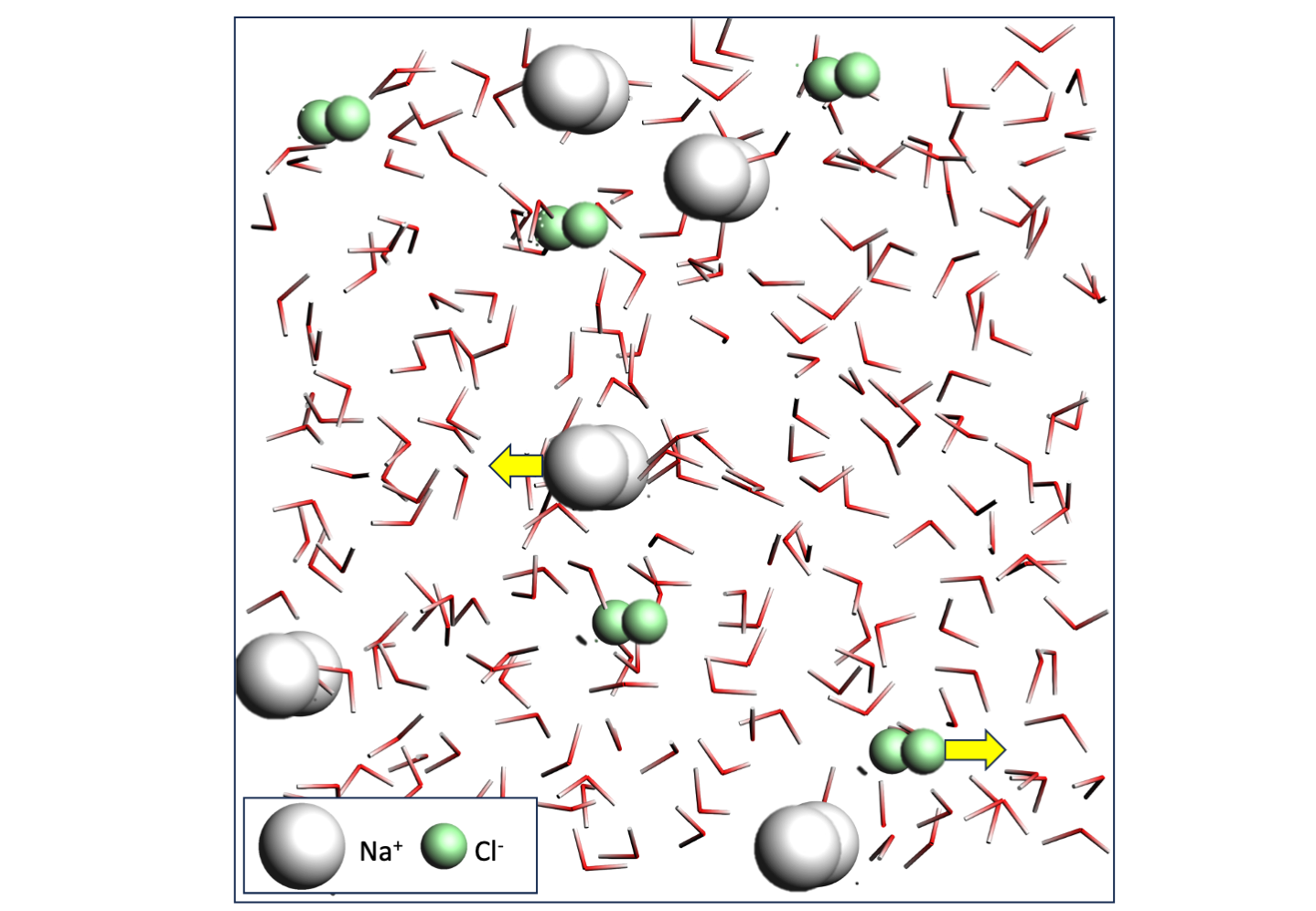
In this tutorial we will compute the ionic conductivity of sodium chloride ions in an aqueous solution by means of molecular dynamics simulations with the ForceField engine.

The system and workflow presented here is very similar to the one described in the publication Estimates of Electrical Conductivity from Molecular Dynamics Simulations: How to Invest the Computational Effort J. Phys. Chem. B 124, 9680−9689 (2020).

	Ionic conductivity (S/m) of 1.21 mol/L NaCl in water at 300K
AMS	7.3
Ref. (MD)	5.9 \(\pm\) 2.9

The tutorial consists of the following steps:

Building a sodium chloride solution with AMBER95 atom types.
Equilibrating the system at 300 K
Running a simulation in the NVT ensemble
Obtaining a value for the ionic conductivity
Comparing that value to literature

If you wish, you can download the already-relaxed sodium chloride solution NaCl_wat.in and jump directly to the diffusion coefficient calculation

Building the NaCl solution¶

Open a new AMSinput window
Switch to ForceField:  → 
Select Type: → Amber95

First we create the building blocks for our system from scratch.

Draw a single Na atom
In the main panel, Click on  next to Atom types
In the column FF Type fill in the AMBER atom type IP
In the column FF Charge fill in 1.0
File → Export coordinates → .in and give it the name “Na.in”

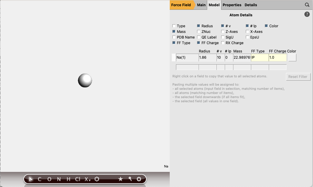
Repeat for a Cl atom (FF Type IM, FF Charge -1.0), and save as “Cl.in”.
Repeat for a single water molecule (FF Types O: OW, H: HW, FF Charges O: -0.8340, H: 0.4170), and save as “h2o.in”.

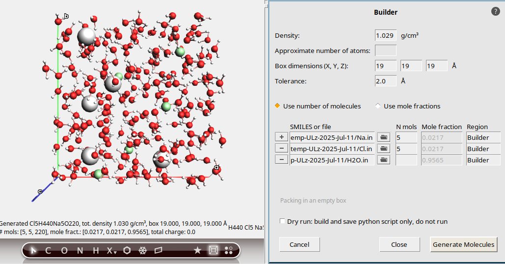
Now we are ready to build the full system.

Remove all atoms from the AMSinput window
Click on Edit → Builder
Make a box of 19x19x19 Angstrom by typing 19 into the diagonal elements of the Lattice vectors
Click on the folder icon next to copies of:, and import the previously saved file “Na.in”
Change the 100 copies into 5 copies
Click on  Molecules: to add a new molecule
Import the previously saved file “Cl.in”, and change to 5 copies
Add a third molecule, import the previously saved file “h2o.in”, and change to 220 copies
Click the Generate Molecules button
Close the Builder tool by clicking the Close button

This should result in an aqueous NaCl solution with a density of 1.029 g/mL.

Important

While building the system, make sure that the Amber95 force field is still selected. Changing the ForceField Type after building will result in all atom typing information being erased.

Equilibrating the system¶

First perform a geometry optimization.

In the main panel, select Task → Geometry Optimization
Periodicity → Bulk
File → Save As… and give it an appropriate name (e.g. “NaCl_optimization”)
Run the calculation
Click yes when asked if the structure in AMSinput should be updated

Equilibrate the resulting system at the desired temperature

In the main panel, select Task → Molecular Dynamics
Click on  next to Task: Molecular Dynamics to go to the MD details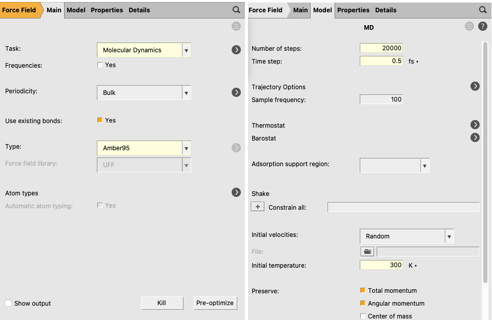
Set the number of steps to 20000
Set the Time step to 0.5 fs
Set the Initial temperature to 300 K

Click on  next to Thermostat to go to the thermostat details
Set the Type to Berendsen
Set the Temperature to 300 K
Set the damping constant to 100 fs

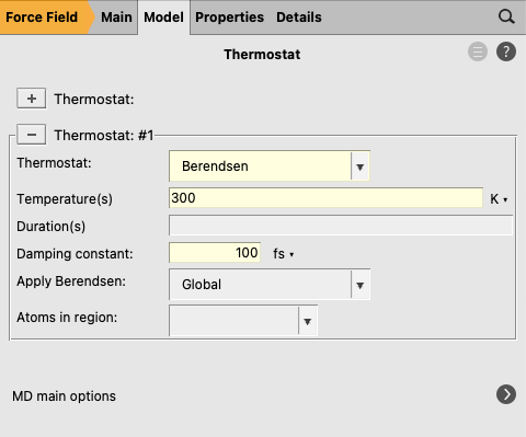
You are now ready to run the simulation.

File → Save As… and give it an appropriate name (e.g. “NaCl_equilibration”)
File → Run
You can follow the progress of the calculation in AMSMovie and AMStail (SCM → Logfile)

AMSMovie can plot the potential energy of the system over the course of the simulation.

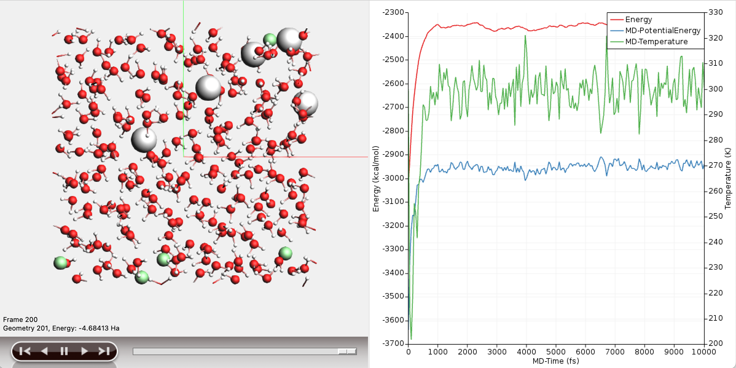
1. In AMSMovie select Properties → Potential Energy

2. In AMSMovie select Properties → Temperature

The potential energy of the system has converged to a stable value over the course of the simulation, and the temperature oscillates around 300K.

Running the Production Simulation¶

When the equilibration calculation has finished, you may be asked whether to update coordinates and bonds. If not, close the NaCl_equilibration AMSinput window, select the job in AMSjobs, and re-open it in AMSinput:

Tick the use MD velocities from results for AMS MD restart box

Select Yes, new job

We will run the production simulation using a Nose-Hoover chain thermostat.

In the main panel, select Task → Molecular Dynamics
Click on  next to Task: Molecular Dynamics to go to the MD details
Set the number of steps to 100000
Set the Sample frequency to 20

If you ran the equilibration yourself:

5. Set initial velocities to From File and set File to the ams.rkf file from the NaCl_equilibration job (if it isn’t set already)

Otherwise, if you simply imported the provided equilibrated structure:

5. Set initial velocities to Random and set Temperature to 300

Then continue with the thermostat settings:

Click on  next to Thermostat to go to the thermostat details
Set the Type to NHC
Set the Temperature to 300 K
Set the damping constant to 100 fs

You are now ready to run the simulation.

File → Save As… and give it an appropriate name (e.g. “NaCl_production”)
File → Run
You can follow the progress of the calculation in AMSMovie and AMStail (SCM → Logfile)

Computing the Ionic Conductivity¶

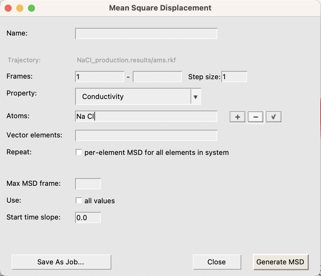
The ionic conductivity is proportional to the slope of the charge weighted mean square displacement of the atoms.

\(\sigma = \lim_{t\to\infty} \frac{1}{2tdVk_BT} \sum_i^N q_i^2 \langle ({\bf{r_i}}(0) - {\bf{r_i}}(t))^2 \rangle\)

Here \(d\) is the dimensionality of the systems (usually \(d=3\)), and \(N\) is the number of ions.

To compute it, open the completed simulation in AMSMovie.

In AMSMovie select MD Properties → MSD
Select Property → Conductivity
Set Atoms to Na Cl
Click on Generate MSD

Two new curves have appeared in the AMSMovie window. The bottom curve depicts the convergence of the ionic conductivity with the correlation time. The final value of the ionic conductivity is 7.34 S/m (or C²/Jms). The corresponding literature states that the value should fall between 1.2 and 13.5 S/m, with an average over many simulations of 5.9 S/m.

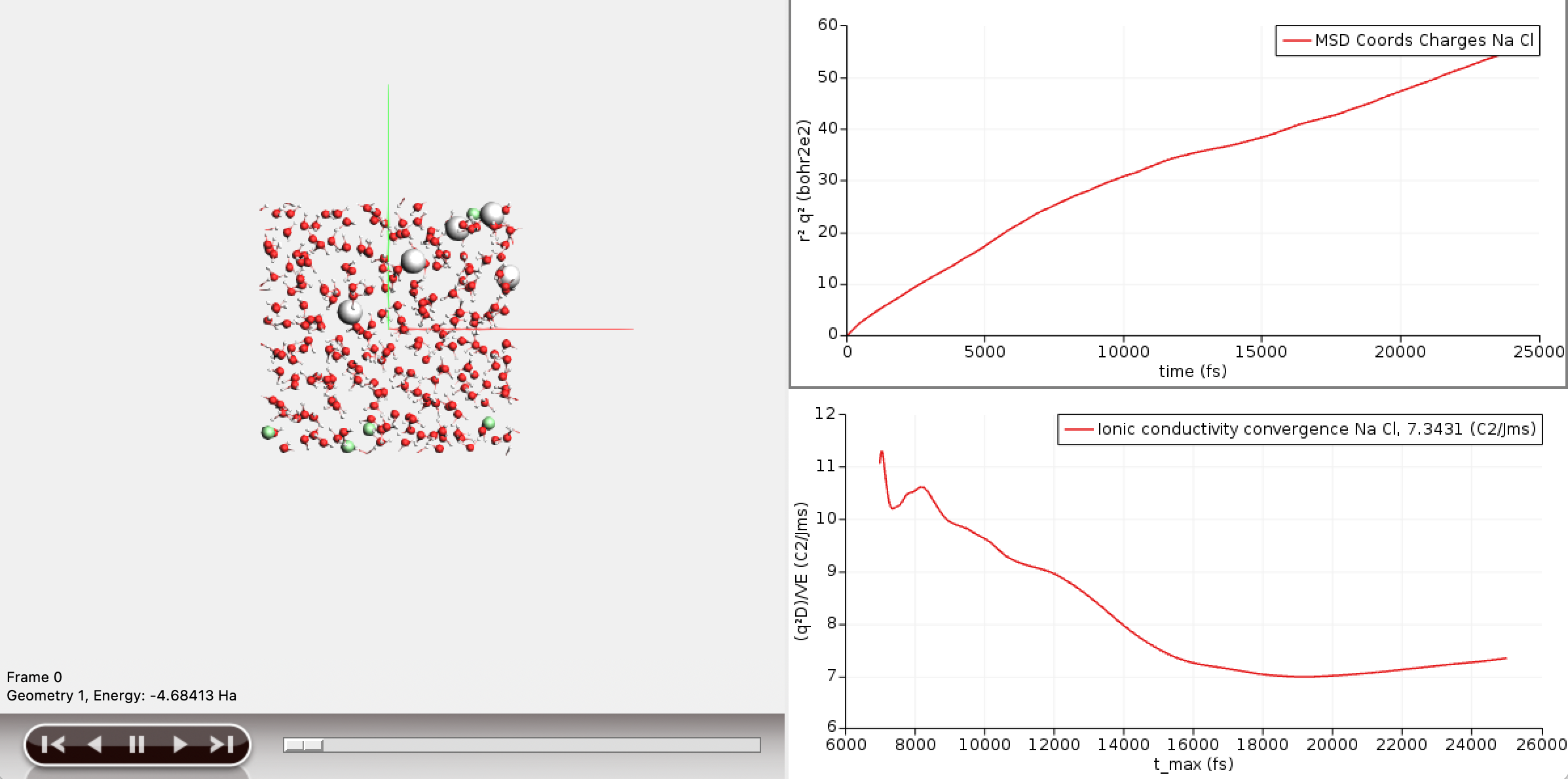
The top curve depicts the charge weighted mean square displacement curve, of which the ionic conductivity is the slope. The graph shows that at short correlation times the slope of the curve is large, and then gradually becomes constant. The point where the curve becomes linear roughly corresponds to the time it takes for the motions of the ions to decorrelate. AMSMovie attempts to estimate this point from the shape of the mean square displacement curve. Indeed, the bottom graph starts at around 7ps, which is AMSMovies guess. However, a brief look at the top curve suggests that a better guess for the decorrelation time would be around 10 ps. We can recompute the ionic conductivity with this new decorrelation time in mind.

In AMSMovie select MD Properties → MSD
Keep all settings the same as before
Set Start time slope to 10000.0
Click on Replace MSD

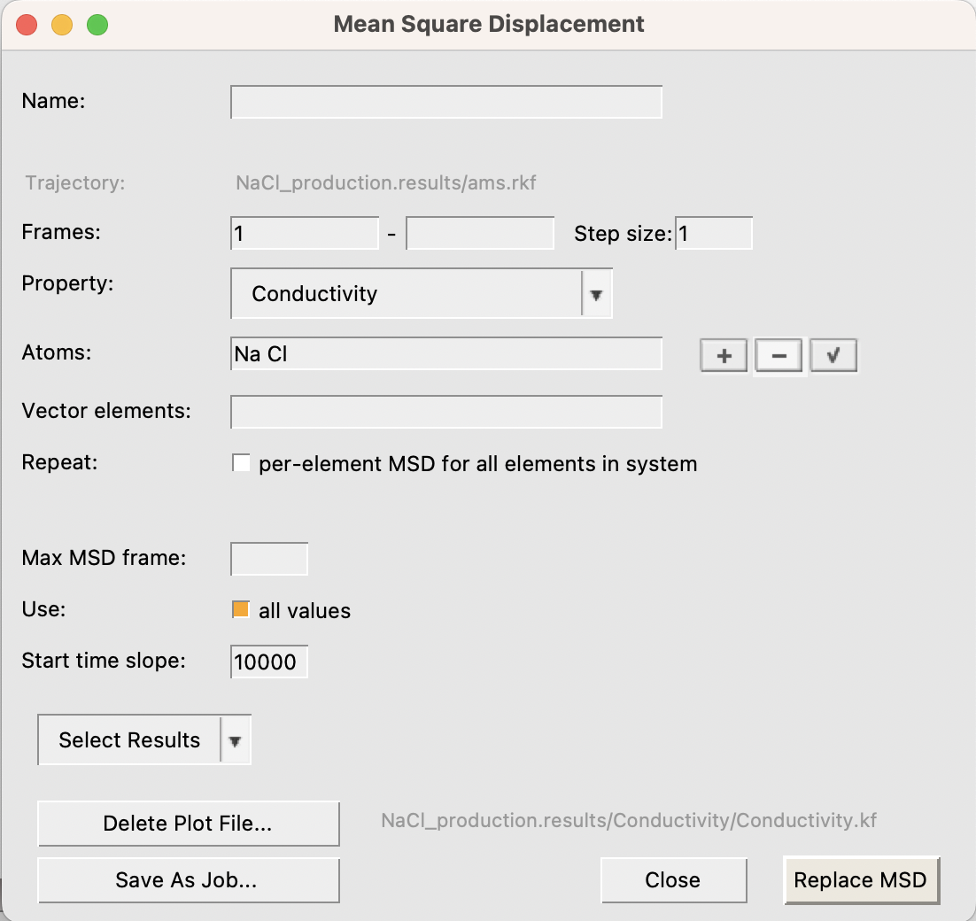
The new value for the ionic conductivity is 7.29 S/m.

Important

The example simulation presented here is too short to obtain really reliable results. In practice it is advised to perform multiple simulations of several nanoseconds each.

Important

The publication J. Phys. Chem. B 124, 9680−9689 (2020) discusses how the exact, correlated, ionic conductivity would include off-diagonal contributions to the mean square displacement.

\(\sigma_{corr} = \lim_{t\to\infty} \frac{1}{2tdVk_BT} \left( \sum_i^N q_i^2 \langle ({\bf{r_i}}(0) - {\bf{r_i}}(t))^2 \rangle + \sum_{i \neq j}^N q_i q_j \langle ({\bf{r_i}}(0) - {\bf{r_i}}(t)) ({\bf{r_j}}(0) - {\bf{r_j}}(t)) \rangle \right)\)

In this example we used high NaCl concentrations to be able to compare with literature values. Indeed, at these concentrations, the off-diagonal contributions can change the value of \(\sigma\) by approximately a factor two. At lower ion concentrations the effect of the off-diagonal contributions will become negligible.

Important

AMSMovie uses the atomic charges as they are stored on the ams.rkf file (in this case the forcefield charges). In this example, the forcefield charges match the formal charges, but for larger ions, this may not be the case, and this will affect the results.