Chemical Vapor Deposition
This tutorial
explains the modeling concepts behind simulating chemical vapor deposition
provides a step-by-step guide on how to set up such a simulations from the GUI
Modeling Chemical Vapor Deposition
From a modeling perspective, chemical vapor deposition (CVD) or atomic layer deposition (ALD) is similar to other processes involving a surface interacting with an atmosphere above it. Further examples of surface-atmosphere interactions include physical vapor deposition (PVD), solid-gas phase heterogeneous catalysis, as well as plasma-surface reactions. As such all of these processes can in principle be studied with setups similar to the CVD example application introduced below.
Caveats
Simulating surface-atmosphere interactions typically involves quite large computations due to the following reasons.
- Model Size
The employed periodic surface models have to feature large unit cells to account for the amorphous structural motifs that result from the deposition of nanometer sized films. In the case of more energetic particles (plasma, sputtering, etc.) impacting the surface, the slab model of the latter needs to be have a certain thickness to account for particle penetration phenomena.
- Time Scale
To model reactions on a surface the time resolution of the simulation needs to be short enough to account for the highest vibrational modes of the system. This time scale is often orders of magnitude smaller than the average interval between successive particle impacts around any given site of the model. When studying atmospheres with low pressures such as those occuring in typical high vacuum surface science experiments, this discrepancy in time scales increases further. Furthermore, surface reactions may involve several intermediate or diffusion steps and require therefore significant simulation times too.
- Pressure
Even with the accelerated dynamics simulations over millions of steps presented in this tutorial, the effective pressures achieved during the simulation are much higher than in reality. While being a compromise, this approach can be justified for cases where the chemical evolution at any given site occurs fast enough to not be affected by successive particle impacts.
- Temperature
The local temperature of the slab model might be raised significantly by either a too strong flux of particles, or even by some acceleration methods. The simulation needs thus to be monitored for temperature spikes and adjusted in order to avoid unrealistic side reactions.
- Evolution
The quality with which a model is described during its simulation is crucial to study a realistic evolution of the system. While the model description of such long simulations is essentially limited to empirical force fields or machine learning potentials, it is advised to carefully parametrize such methods for relevant reaction steps prior to begin any production simulations. While the example discussed below simulates realistic chemical processes with an existing ReaxFF parametrization, this cannot be assumed in the general case. Especially, relative discrepancies in reaction barrier heights can affect the chemical processes occurring during the simulation and significantly alter the evolution of the system. It is therefore the responsibility of the user to use adequately validated model descriptions for the simulations in interest. The ParAMS tutorials and documentation provide further information on how to obtain such parameterizations.
Model
The model used in the CVD simulations is sketched below and features the following components

Fig. 27 Sketch of the CVD simulation model: particles are inserted in a box (orange) and translated close to their first impact point, where they are actually placed into the simulation box. From there, a particle can either be adsorbed on the surface and undergo further reactions there (blue), or either be reflected (red) or penetrate through the surface (green). In either of the latter cases, it will leave the safe box (dashed line) and be removed.
- Mechanical Properties
Our model mimics a surface with an underlying bulk, and should therefore have a similar mechanical resistance to particle impacts. This is achieved by fixing all atoms in a mechanical support layer at the bottom of the slab model.
- Thermal Properties
The model should also approach the thermal properties of the underlying bulk material while still allowing for local hotspots around particle impact sites. This is implemented by adding a thermostat module affecting only atoms in another layer deep below the surface, directly above the mechanical support.
- Molecule Gun
Particles are (formally) inserted in a random position within a zone located several nanometers above the surface and with a velocity vector pointing downwards.
- Particle Translation
To save simulation steps during the particle flight time, the particle is translated close to the first impact point in its flight path. It is then actually placed into the simulation box near this impact point.
- Accelerated Dynamics
In regular intervals timed to start directly after each initial particle contact with the surface, a sequence of accelerated dynamics steps using the force-bias Monte Carlo method commences.
- Molecule Sink
If a particle moves away from the surface, it will likely not interact with any other parts of the model either. A safe-box is defined encompassing a large region around the entire surface model. If any stray particle leaves the safe box it is automatically removed by the molecule sink module.
Simulation Setup and Settings
Oxidized Ge(001) Surface
The slab model was obtained from a crystal Ge structure, whose lattice parameters were optimized with the ReaxFF parametrization CHOFeAlNiCuSCrSiGe.ff used in all subsequent simulations.
After converting the crystal to a surface slab model, the oxygen centers were added to the surface and relaxed in the following.
We refer to the crystals & surfaces tutorial for details on building such slab models and provide the initial structure of the partially oxidized Ge(001) surface as an xyz-file for download.
xyz file of the partially oxidized Ge(001) slab modelRegions
With the initial model imported, we begin by setting up the mechanical support and thermostat layers in the model:
 and name the new region as fixed
 and then change to Model → Geometry Constraints and PES Scan, select one atom from the fixed region fixed (fixed position)
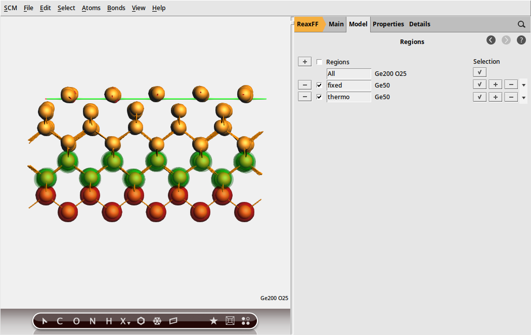
Fig. 28 Mechanical support and thermostat layer as regions used in the simulations
Equilibration
We can now set up a short simulation to equilibrate the system to the temperature used in the following calculations.
and select Force Field: CHOFeAlNiCuSCrSiGe.ff
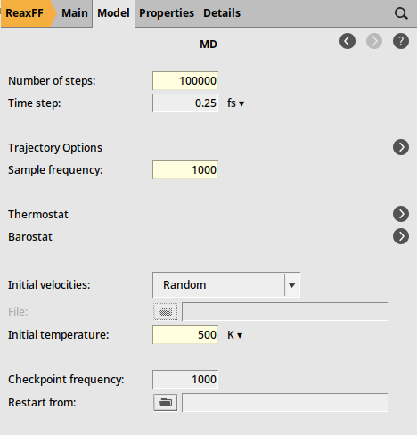
Fig. 29 Molecular dynamics settings
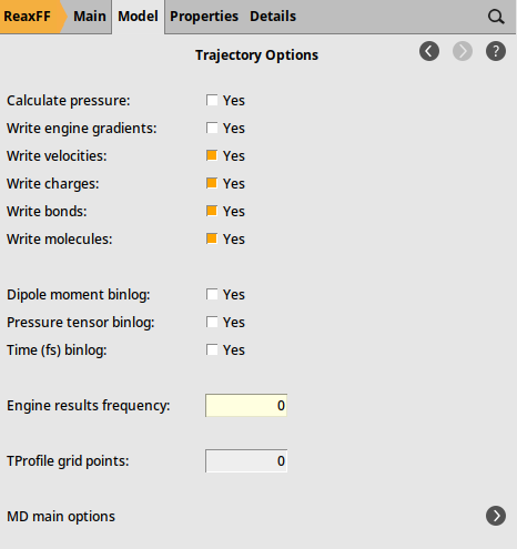
Fig. 30 Trajectory sampling settings
next to it to add a thermostat instance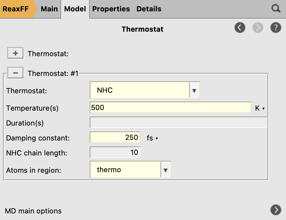
Fig. 31 Thermostat settings
While the above settings suffice to equilibrate the system in principle, we would also like to include the effect of the accelerated dynamics phases used in the main simulation. Indeed, the employed force bias Monte Carlo method is known to accelerate the evolution of a system by violating the reversibility of larger Monte Carlo steps. For this reason, we activate the fbMC module already for the equilibration run:
to add a new fbMC instance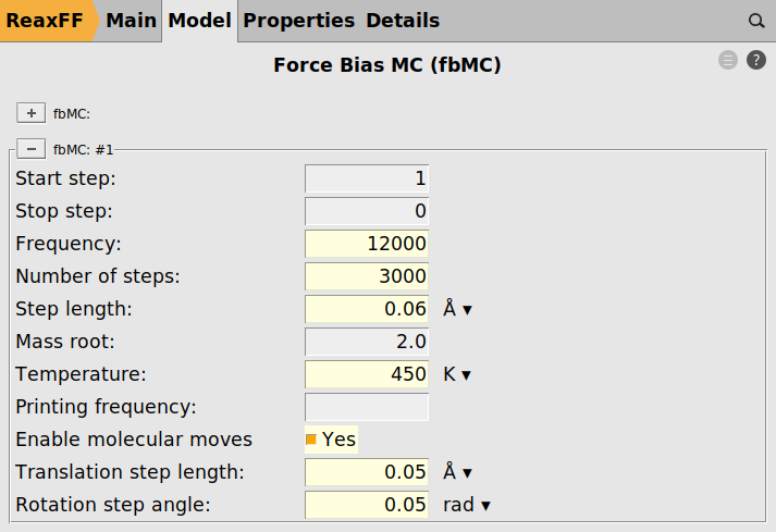
Fig. 32 Force bias Monte Carlo settings
Note
We deliberately use a slightly lower temperature during the fbMC phase than for the thermostat, 450 vs 500 K, to avoid too high temperature spikes during the simulation. This choice is justified as we are interested in the general chemical evolution of the system. In addition, because the impinging particle flux adds energy to the system, keeping the temperature stable is deemed more important in this situation than a precise thermodynamic sampling. In other applications, the effect of the fbMC temperature and the fbMC step length on the temperature actually observed need to be validated by the user.
Simulation
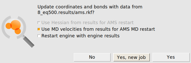
Using the equilibrated positions and velocities allows now to set up the production simulation. We load
after the above equilibration run is complete
Warning
Make sure that the original job and the ams.rkf result file is not overwritten
For convenience, we provide the input file for the equilibration run, Ge200O25_equilibration.ams, as well as the resulting Ge200O25.rkf file containing the equilibrated Ge(001) surface structure and atomic velocities for download.
Note
In newer versions of AMS, the regions are imported from the .rkf file. If the regions fixed and thermo are not present after importing the coordinates, either update AMS or repeat the steps in the above Regions subsection.
After either of these steps, we can start setting up the final simulation run. We begin with adapting the settings for MD and fbMC
Note that the above Start Step settings are used to align the start of the fbMC intervals with the molecule gun shots.
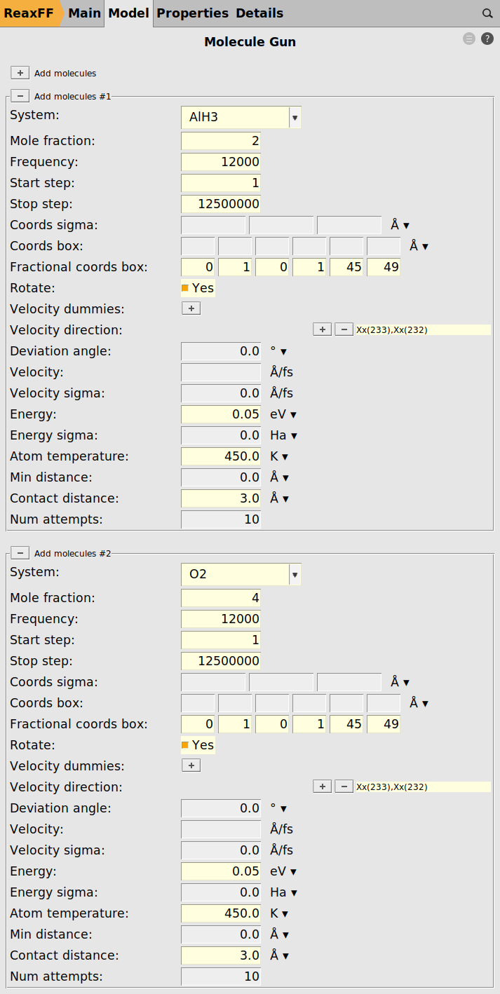
We proceed by loading the structures for the O2 and AlH3 projectiles.
These are provided in the files O2.xyz and AlH3.xyz for download.
We can now use these imported regions as O2 and AlH3 projectiles in the molecule gun module.
to add a new projectile, and select the top dummy atom followed by the lower oneTo add the O2 projectile
to add a new projectileNote
Except for Mole Fraction, the settings have to be identical for both projectiles as shown in the figure below
Note
The Stop Step setting is used to realize an annealing phase at the end of the simulation
As a last step, we enable the molecule sink to remove any stray particles from the model.
next to “Remove molecules”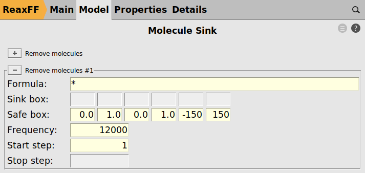
We are now ready to start the simulation using File → Run.
For the readers’ convenience, we provide the input file for this calculation, Ge200O25_O2_AlH3_fbMCCVD.ams, as well as the previous equilibrium simulation result, Ge200O25.rkf. Afterwards, we just need to follow the steps below to manually set up the initial velocities.
Warning
Due to the nature of the simulation, the calculation will run for an extended time. Depending on the hardware available, several days of runtime should be anticipated.
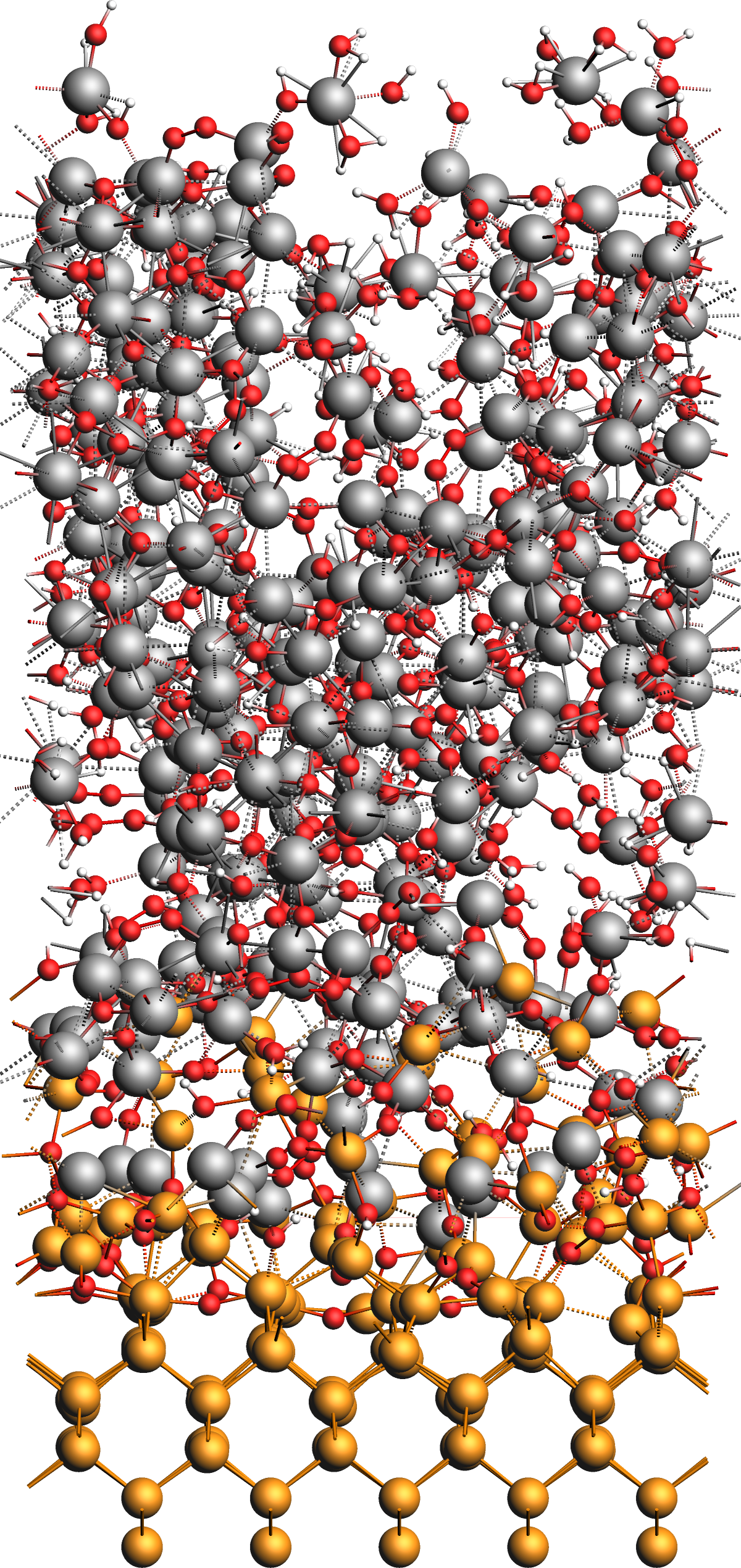
Results: Alumina Film on Ge(001)
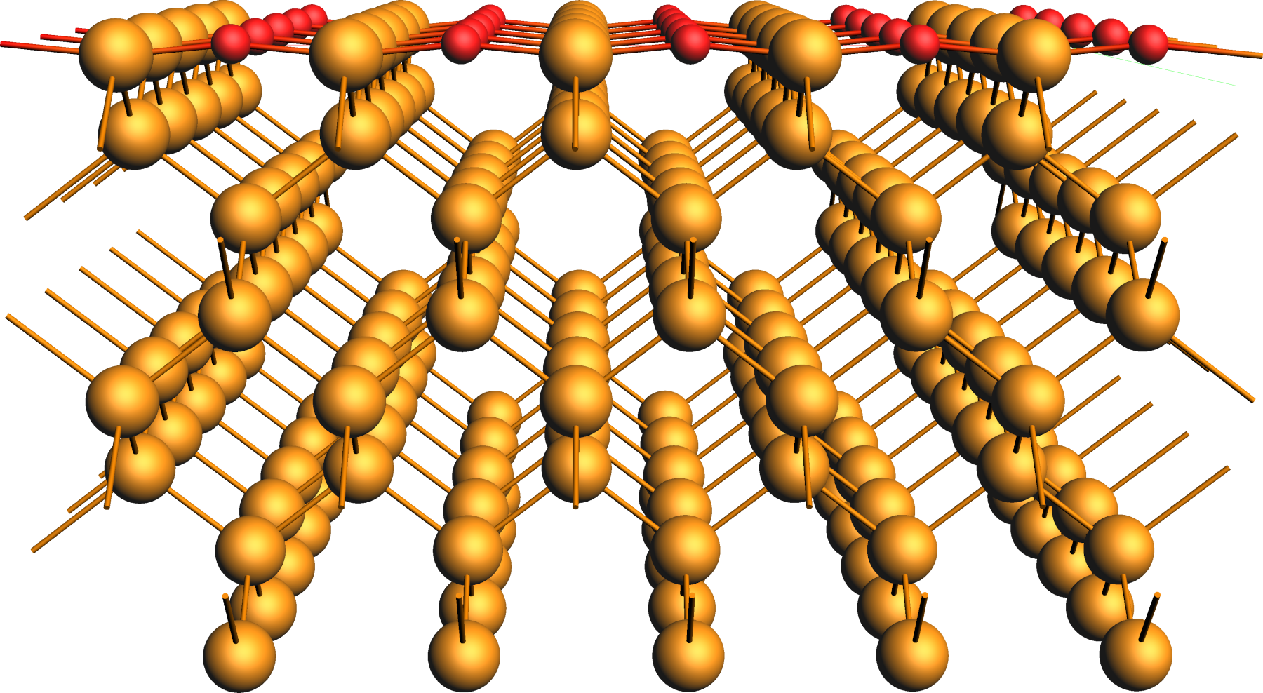
After the simulation, we obtain the model structure shown in the figure below. The original surface is covered by an amorphous interface layer followed by a thick but loose and alumina film with many absorbed water molecules and OH groups as well as several chemisorbed aluminum complex moieties on the surface of the film.
We conclude this tutorial by noting several observations from the results:
- Deposition Process
During the CVD simulation, the projectiles can be observed to appear just above the surface, getting absorbed to either react or desorb later, or getting reflected immediately. On average, more projectiles end up bound to the surface, which creates an amorphous alumina film growing over time.
- Energy and Temperature
Consequently, the total energy of the system is continuously lowered as more chemical bonds are formed. In the beginning of the simulation, we observe strong temperature fluctuations, which gradually decrease over time. This latter observation is the result of an initially small model whose temperature can be easily affected by impinging particles.
- Model Size
As this tutorial includes lengthy calculations, we opted for reducing the model size. In scientific studies, the use of a deeper and wider slab model might be more appropriate.
- Alumina Film
Depending on the exact simulation condition (temperature, particle flux, particle kinetic energy etc.) films with different properties emerge. E.g. increasing the temperature generally reduces the water content in the film while increasing its density. The mole fraction of the flux of particles can affect the deposited film too. To obtain a clean alumina film, it is advisable to use an excess of oxygen during the deposition.
- Ge(001) surface and interface
We generally observe the germanium surface to remain intact without any of its atoms desorbing. The interface between the germanium and alumina layers forms from an GeAl alloy layer, which in turn originates from the interaction between the AlH3 particles and the clean surface. With increasing oxidation, the deposited film separates into a mostly pure alumina film and an GeAl alloy interface layer. Depending on the exact conditions, small alloys clusters are also be observed to move on top of the film during the phase separation.