eReaxFF: Electron transfer in MD

Overview

The novel eReaxFF method is an extension to the well-known reactive force field ReaxFF. It allows for the simulation of explicit electrons within the ReaxFF framework. Those electrons are treated in a pseudoclassical manner that is orders of magnitude faster than any quantum chemical methods.

In this tutorial, eReaxFF is used to simulate the dynamics of an electron transferring through a hydrocarbon radical. A detailed description of the eReaxFF method and the carbanion (explicit electron + hydrocarbon radical) are given in:

Md Mahbubul Islam, Grigory Kolesov, Toon Verstraelen, Efthimios Kaxiras, and Adri C. T. van Duin, eReaxFF: A Pseudoclassical Treatment of Explicit Electrons within Reactive Force Field Simulations. , J. Chem. Theory Comput. 2016, 12, 8, 3463–3472.

This tutorial was also featured in our video tip of the week series

This tutorial assumes a basic familiarity with the GUI. If you are not familiar with using the GUI yet, you might take a look at the GUI introduction tutorials before continuing.

The System

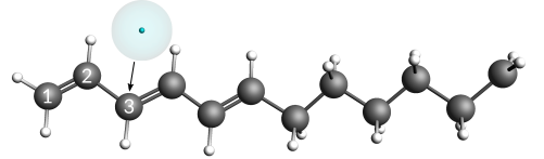
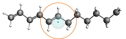
The hydrocarbon radical C₁₂H₁₉• is the base used to construct an anion with one explicit electron. This radical consists of both a conjugated (polyacetylene) and an aliphatic part. In addition, a radical site has been placed on the end of the aliphatic part (labeled CH₂in the below image).

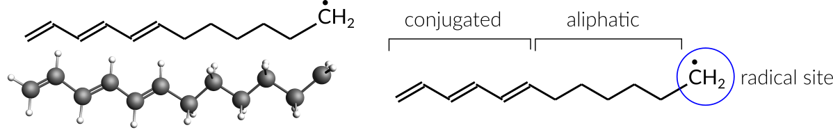
An excited anion is generated by inserting one explicit electron into the conjugated part of the radical. From there the electron can diffuse through the chain until eventually settling at the radical site. Once the electron settles at the radical site, the ground state of the anion, a primary carbanion, is reached.

Setting up the MD simulation

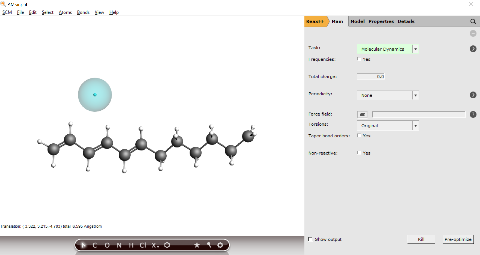
Begin by importing the radical structure into AMSinput

1. Download the file C12H19.xyz here

2. In AMSinput: File → Import Coordinates

3. Select the XYZ file you just downloaded using the file dialogue window

4. Change to the ReaxFF panel,

Next, add the explicit electron to the system

1. Click on the Element tool

2. From the periodic table, select El

1. Place the electron next to the radical

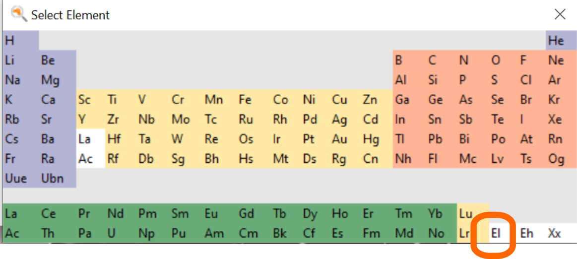
Before placing the electron in its final position, create a new region and add only the electron to that region.

1. Go to Model → Regions

2. Select the electron in the view panel

3. Click on the Add button

4. Name the region ‘El’

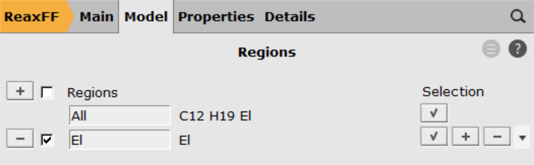
Using the newly created region (El), define a charge constraint that will ensure the electron particle remains its charge of -1 throughout the charge equilibration scheme

1. Go to Model → Charge constraints

2. Click on the Add button,

3. Select the region El and enter -1 into the Charge field.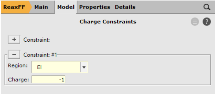

Next, move the electron particle onto its final starting position, which is very close (5 pm) to carbon atom #3.

Placing the electron and carbon atom almost on top of each other at a defined distance is best done by using the distance slider of the GUI.

1. Select the electron in the view panel

2. Hold down the SHIFT key and select carbon atom #3

3. Use the distance slider or the entry field to set a distance of 5 pm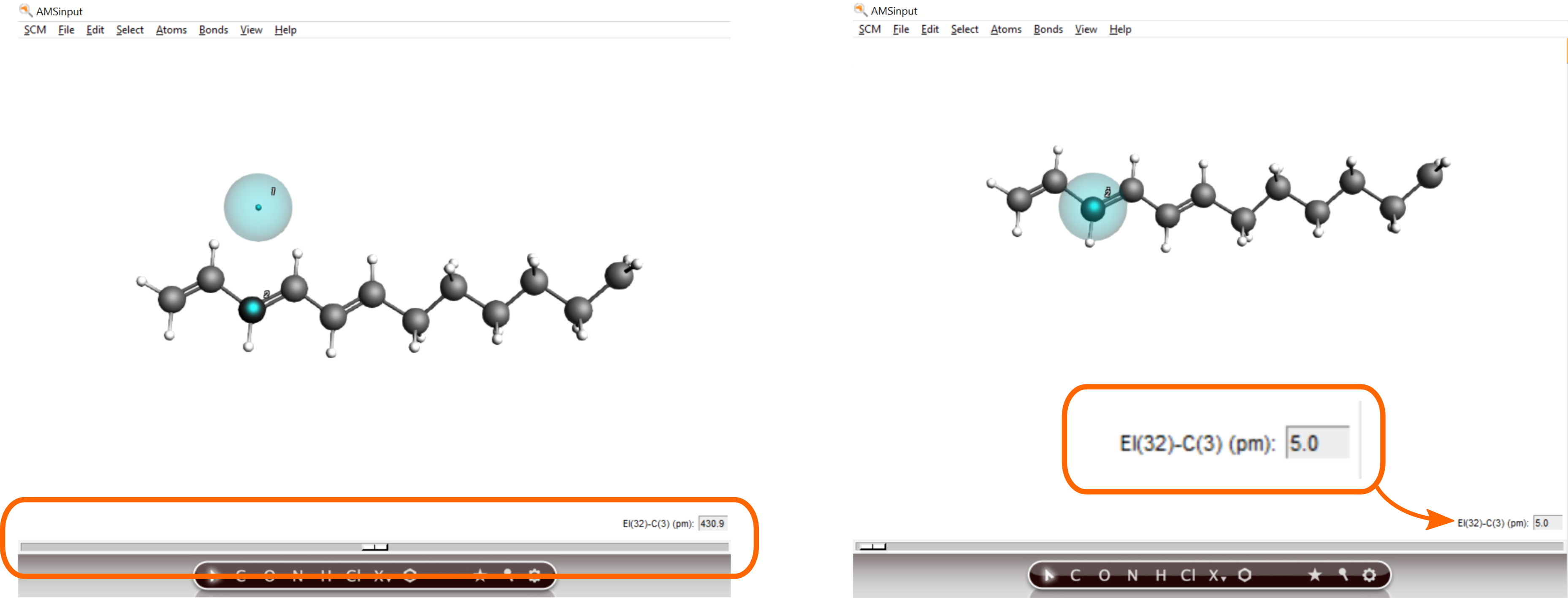

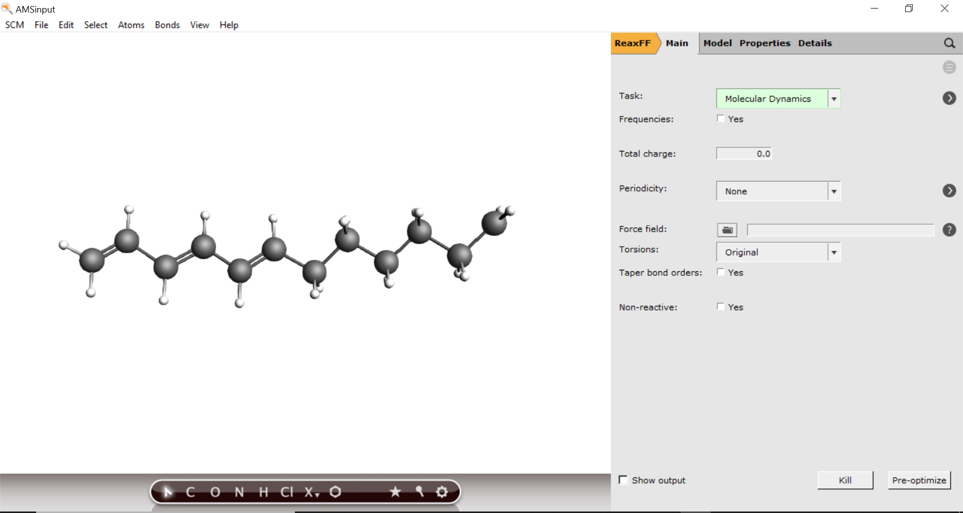
Now, only the general ReaxFF and MD settings need to be setup.

1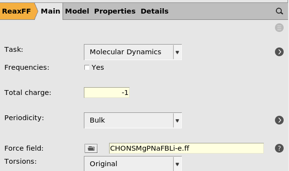. In the Main panel

2. Set Total charge to -1

3. In the Force field drop-down, select CHONSMoNiLiBFP-e.ff.

Move on to the general MD settings

1. Click on next to Task: Molecular Dynamics

2. Enter Number of steps 750 000

3. Enter Time step 0.1 fs

4. Enter Sample frequency 500

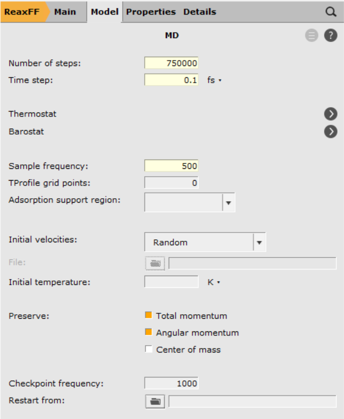
And finally, define the thermostat and start the calculation.

1. Click on next to Thermostat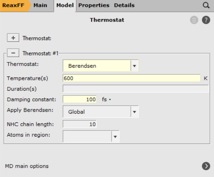

2. Click on the

3. Select Thermostat → Berendsen

4. Set Temperature to 600

5. Set Damping constant to 100 fs

6. Save and Run. (Ignore a potential warning about atoms being too close.)

The progress of the simulation can be followed in AMSmovie.

Analyzing the results

Note

This simulation depends on random numbers, therefore your results may differ from the ones discussed here. The general trend should be reproduced. More information on the results are found in Md Mahbubul Islam, Grigory Kolesov, Toon Verstraelen, Efthimios Kaxiras, and Adri C. T. van Duin, eReaxFF: A Pseudoclassical Treatment of Explicit Electrons within Reactive Force Field Simulations. , J. Chem. Theory Comput. 2016, 12, 8, 3463–3472.

The qualitative analysis of the results can easily be done in AMSmovie:

1. Click on the SCM menu and select Movie

2. Start the playback by clicking on the play button

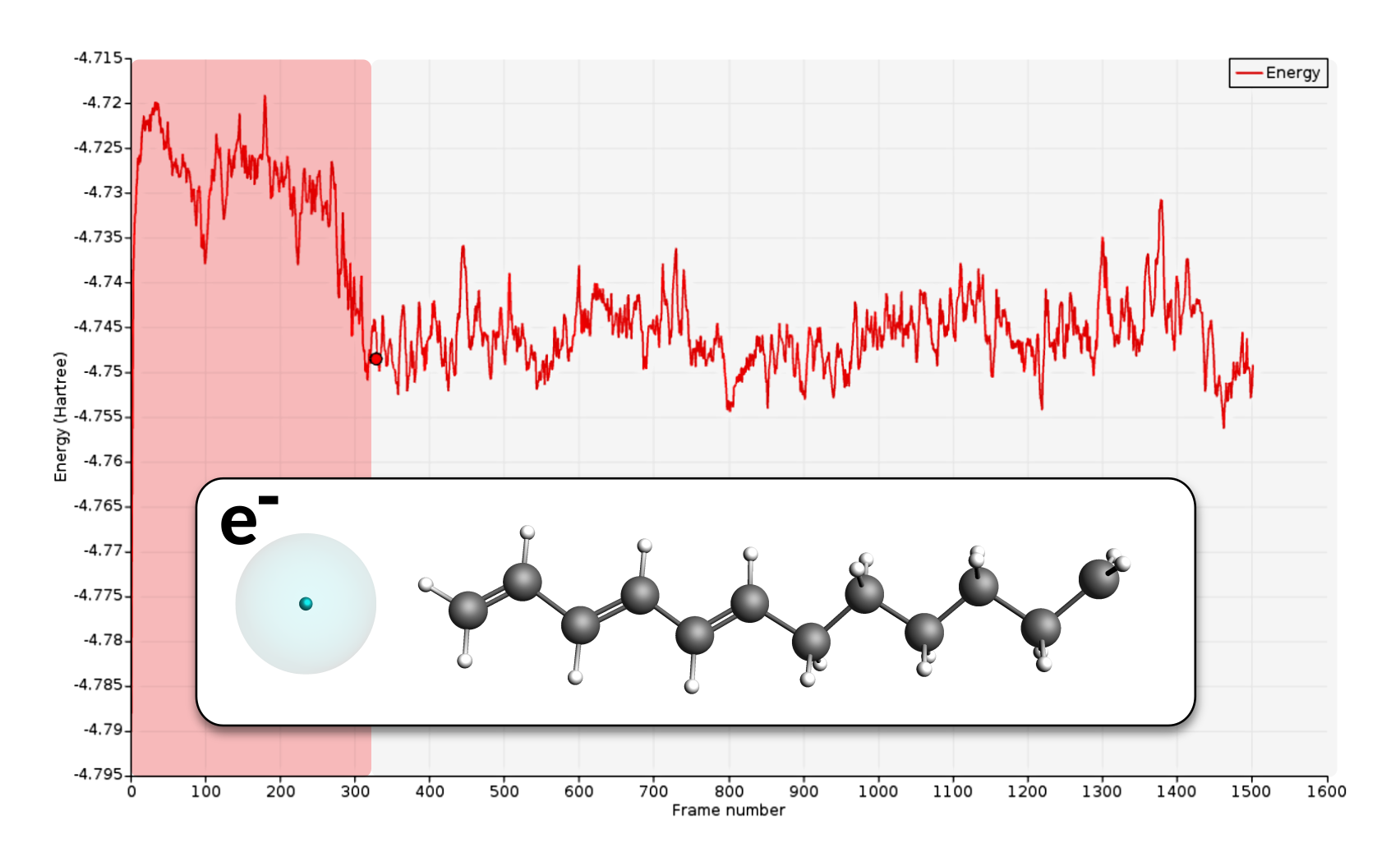
You should see the electron diffusing through the hydrocarbon radical. The electron diffuses rather effortlessly through the conjugated chain, while the intersection between the aliphatic and conjugated parts is a point with slightly higher stability. This slightly higher stability is the reason why the electron is often seen in the vicinity of this region.

Eventually, the electron will be able to escape the small well at the intersection region and diffuse to the radical site. The arrival at the radical site, i.e. ground state, is clearly visible as a drop in the total energy of the system.

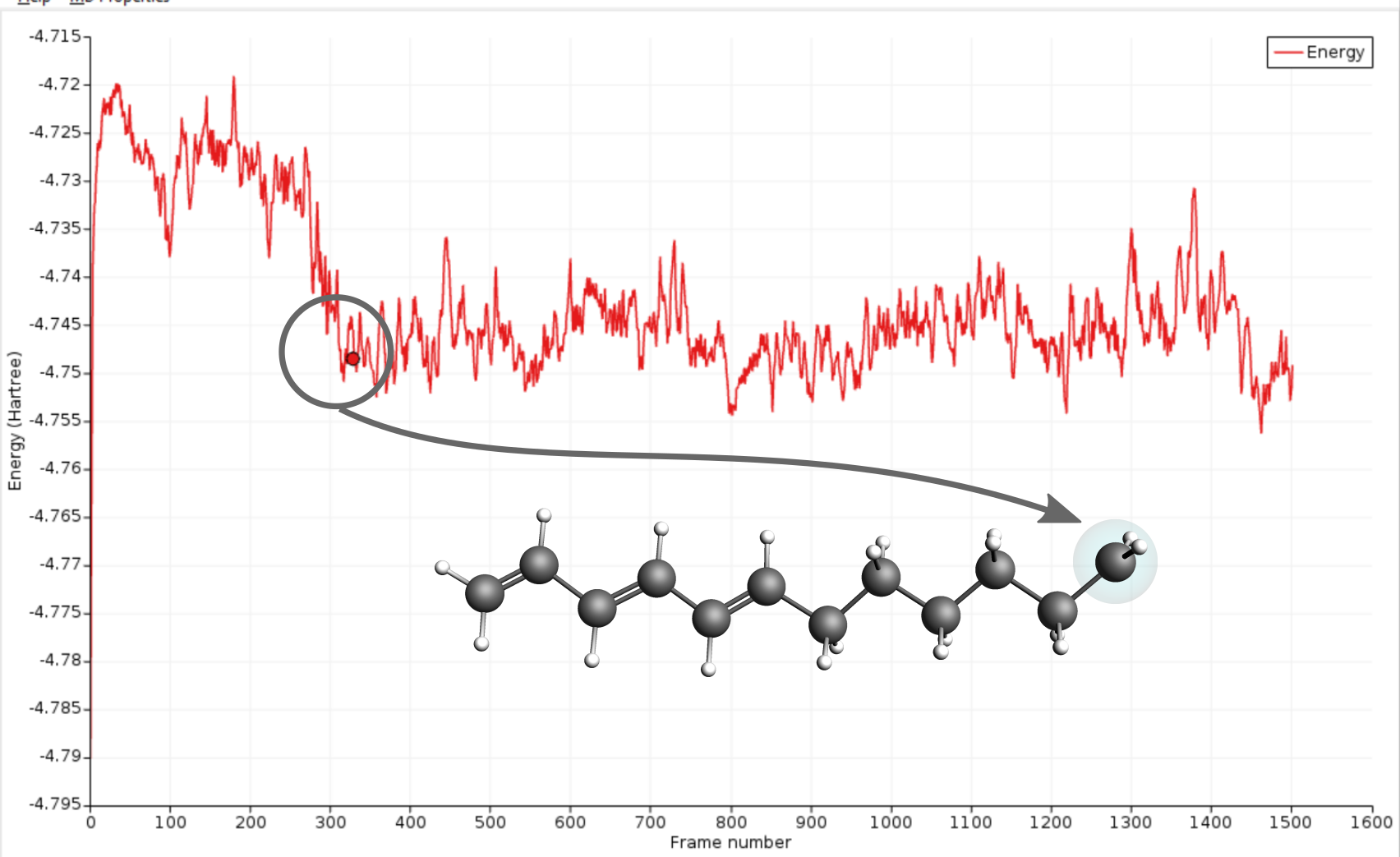
In the present case the electron transfer to the radical site took around 275 frames which correspond to 13.75ps. Compared to the literature reference this is faster than average but as mentioned in the beginning of this section, different runs will yield different results due to the use of random numbers.

A more quantitative analysis can be carried out by comparing transfer rates at different temperatures and/or calculating a time averaged position of the electron along the atoms of the chain. The transfer times can simply be extracted from the movies of different trajectories, while the calculation of averaged positions is easily done with the help of the PLAMS python library shipped with AMS