ChemTraYzer2: Reactive MD Analysis
Introduction
Molecular dynamics (MD) simulations are a common way to simulate the time evolution of larger chemical systems. Because MD is often based on classical mechanics, systems can comprise thousands of interacting atoms, making it possible to study a variety of physical and chemical phenomena.
When simulating a reactive system – where chemical bonds between atoms can change over time – it is not uncommon to observe a very large number of reactions. For large or complex simulations, the many reactive events make it challenging to derive meaningful information from the trajectory. ChemTraYzer2 (CT2) is a tool designed to help with this problem. CT2 reads each frame of a reactive MD trajectory, keeps track of all reactions that occur, and summarizes all of this information into several useful quantities: a list of unique reactions, reaction rate constants for these reactions, the net fluxes of each species encountered in the simulation, and other kinetic and population measures.
See also
Summary of this tutorial
With this tutorial, we show how to:
set up a typical reactive gas simulation with a lot of reactions
run the molecular dynamics simulation with the ReaxFF engine
set up ChemTraYzer 2 in the AMS GUI
find the reactions of the simulation
get rate constants for those reactions
visualize single reactive events in detail
We will start by setting up a common reactive molecular dynamics (MD) simulation. In our case we will simulate the combustion of hydrogen in a stoichiometric hydrogen/oxygen mixture, following this balanced reaction equation:
Of course, hydrogen and oxygen will not react directly in this way, but rather via some intermediates like \(\mathrm{H}\), \(\mathrm{OH}\), and \(\mathrm{HO_2}\), for example, by these elementary steps:
For this tutorial, we will choose an extreme temperature and density, because then the combustion reactions will happen faster and we can observe them within the time for this tutorial. When burning hydrogen, some types of reactions are expected to happen, like oxidation of hydrogen and decomposition reactions of oxidated products (as shown above). High temperatures usually favor decomposition pathways, but since we will have a lot of small molecules, we can expect to observe both oxidations and decompositions. Apart from that, the number of hydrogen/oxygen atom combinations in the molecules is quite limited and the resulting reaction network will not explode in size, even though we will simulate in those wild conditions.
Step 1: set up a reactive hydrogen / oxygen combustion simulation
 →
→ 
Building a periodic box of gas
To build our periodic box that contains our gas mixture, we will use the Packed Molecules builder tool of AMS. The builder tool helps us to set up a initial stoichiometric composition and distribute our molecules in the box. We will simulate in quite a small box, so that the runtime of our simulation will be short.
Note
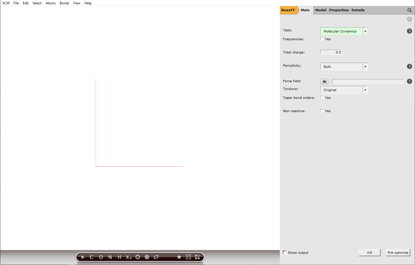
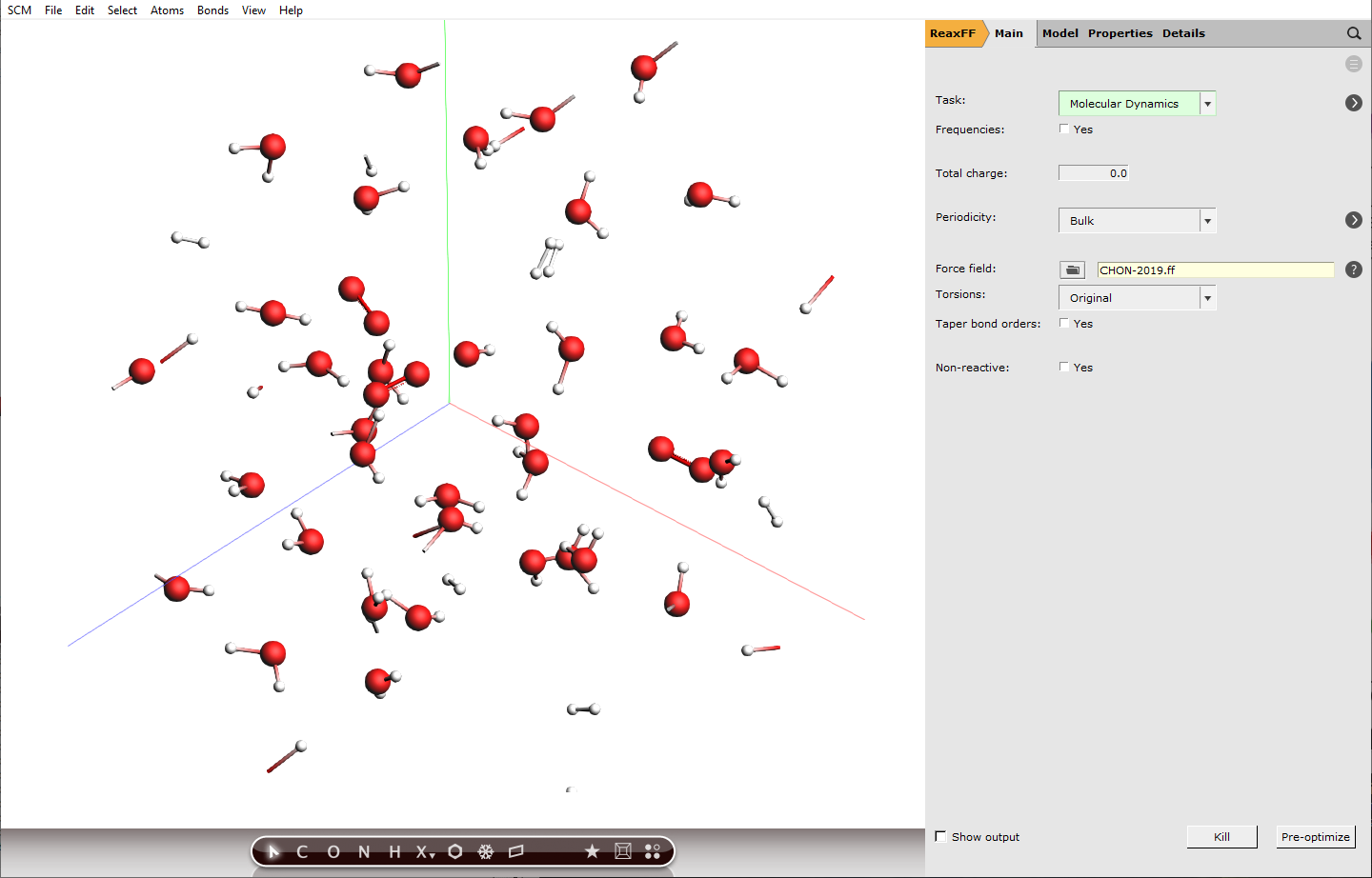
By selecting ReaxFF, molecular dynamics of a periodic box is chosen as a default setting.
15 15 15 Å20 to add a line for another species
40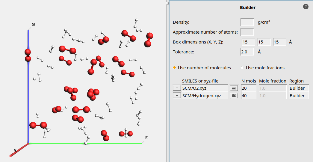
Choosing simulation conditions
With the Builder tool, we already set the density of our system to \(60 / 15^3 \mathrm{molecules/{A^3}}\) which translates to \(29.5 \mathrm{kmol/{m^3}}\). So together with a very high temperature, we will create supercritical conditions, to make the combustion reactions happen faster. This will definitely not be a realistic setup, but it helps to see some reactions within a short calculation time.
Furthermore, we will use the default integration time step of 0.25 fs. With extreme conditions like in our case, the chemistry will be fast and usually smaller integration time steps are recommended to capture the molecular vibrations correctly. However, this would also increase the computation time, which is why we stick to the default value.
 next to Task: Molecular Dynamics
200000103500 K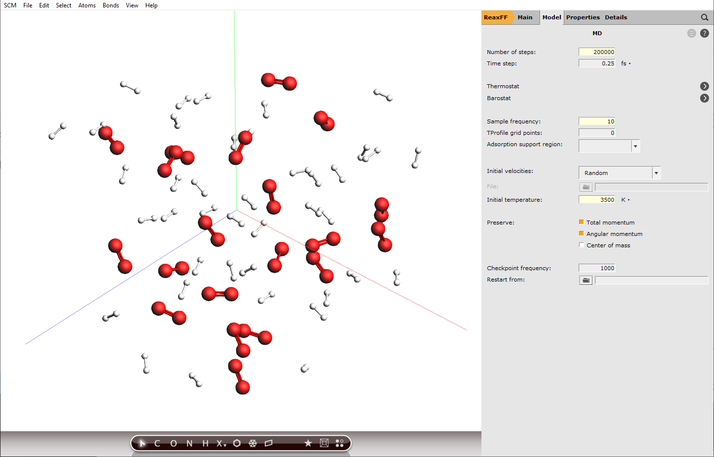
Setting the sample frequency to 10 means every 10th calculated step is written to disk and can be analyzed later, this translates to a time difference of 2.5 fs between frames. Decreasing this value will increase the accuracy of the analysis later, but also the disk usage.
Note
200000 calculation steps at a step size of 0.25 fs translate to 50 ps of simulation.
Setting up a thermostat
ChemTraYzer 2 can calculate rate constants for all observed reactions, by evaluating the number of events and the concentration of reactants for each reaction. The computation assumes constant temperature (an NVT ensemble), which is why we need to set up a thermostat that balances out temperature changes once reactions start to happen.
next to Thermostat and select NHC from the dropdown next to Thermostat:3500 K10 fs
Step 2: Run the simulation with ReaxFF
Note
The list of ReaxFF parameterizations that appears when you click the folder button, will always contain parameters for the elements that are currently in the box.
Tip
Before actually running the simulation, we can check our settings. Details → Run Script summarizes the calculation job that is fed to the AMS calculation engine. All settings which are not default values are listed here. If we forgot to set a crucial setting, the program will notify us here with a pop-up warning.
Running this calculation takes approximately 10 minutes. You can do the following steps while the job is running.
AMSjobs should come to the foreground, and your job should be visible at the top. On the right side you can see that the job is running (this is indicated by the gear-icon). When running, in the AMSjobs window the progress of your simulation is showing (from the logfile). When you click on the progress lines the logfile will open in its own window:
As you can see in the logfile, the simulation is running. To see more details, we now will use AMSmovie. Note that you can do this while the simulation is still running!
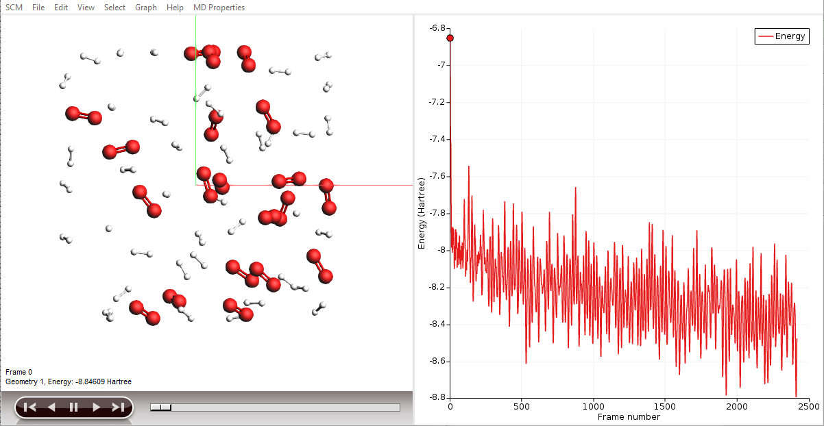
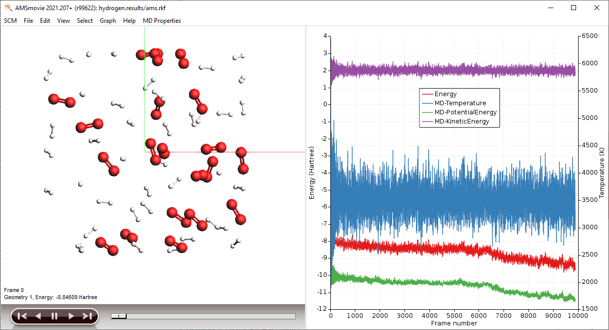
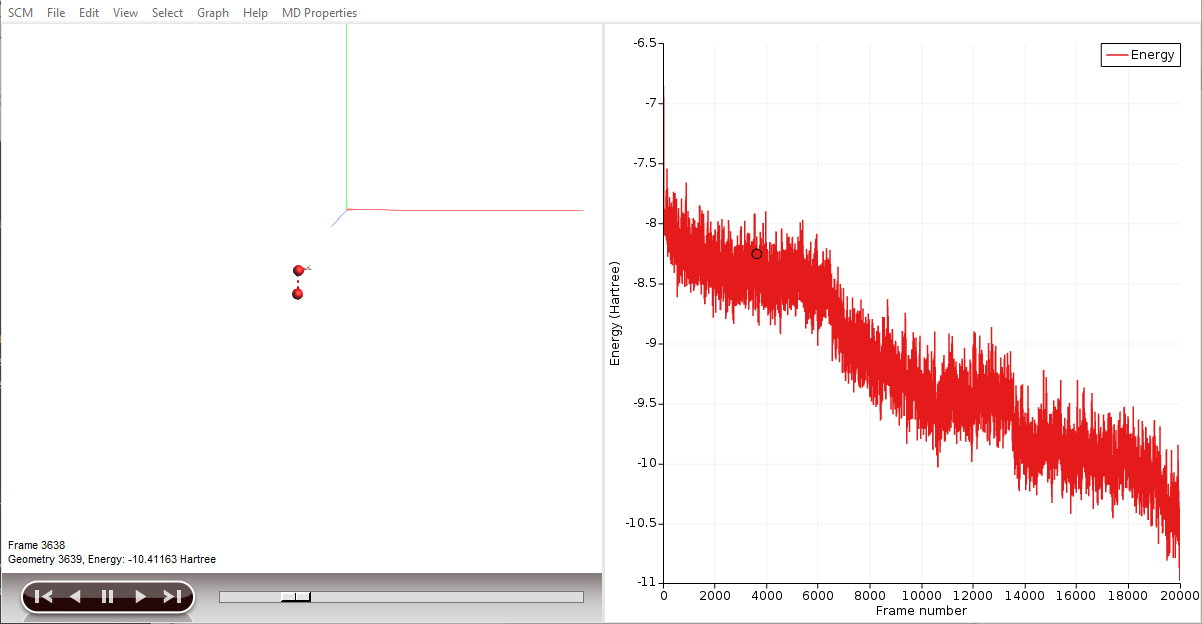
AMSmovie will show you the trajectory of your system. Note that it will automatically read new data as soon as it becomes available. It can also show graphs of the properties that ReaxFF calculates:
Note
When reactions break up bonds, energy is released that was previously chemically bound. As a consequence, the kinetic energy of the system increases and the potential energy decreases. If we had not applied a thermostat, the temperature would rise together with the kinetic energy. The thermostat however slows down each atom from the system while it is heating up, which is why the temperature stays constant and the potential and total energy decrease.
Tip
You can drag the legend in the plotting area around with the mouse
You can go to a particular point in the simulation using the slider below the window showing your system, or you can click somewhere on one of the curves plotted. You can also use the arrow keys (left and right) to move through the simulation. Jump to the end of the movie to follow the progress.
Step 3: Extract a list of reactions with ChemTraYzer 2
To start with this step, first wait for the calculation to finish.
In the AMSlog window you can see the number of calculated steps, which eventually reaches 200000. In AMSmovie, go to the last frame and take a look at the molecules: some new species should have appeared, like \(\mathrm{OH}\) and \(\mathrm{H_2O}\). We didn’t put them in, so they were formed by reactions.
Note
ChemTraYzer 2 can analyze any periodic gas calculation done with ReaxFF. Just open the RKF file in AMSmovie, and start ChemTraYzer 2 as explained below.
Let us see if we are able to find the types of reactions we expected in the beginning.
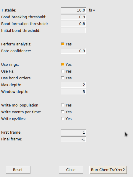
A new window opens with settings for the trajectory analysis by ChemTraYzer 2. At first, we want to keep the standard settings as they are.
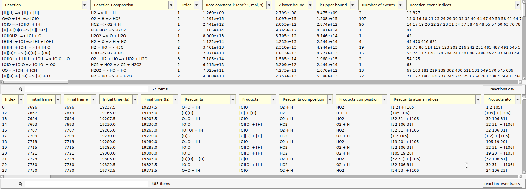
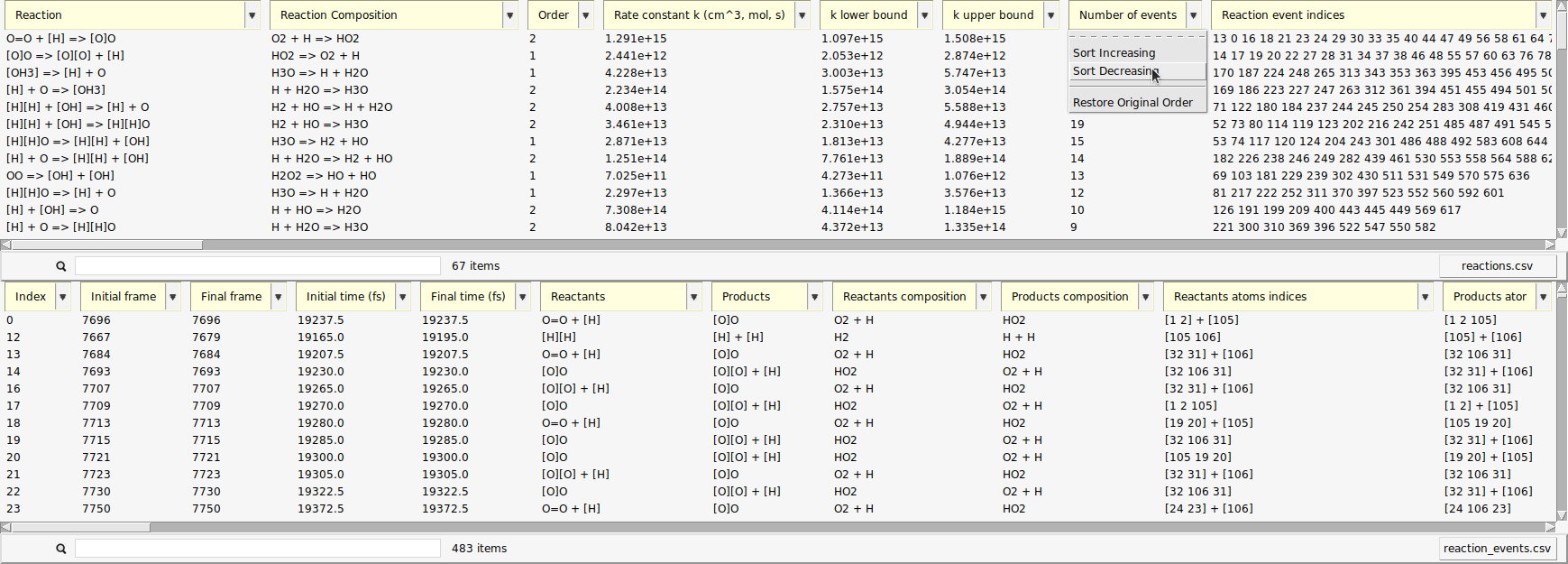
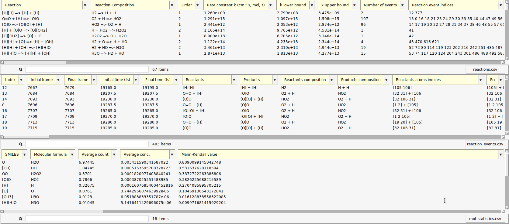
A new window opens with a list of the reactions found by ChemTraYzer 2. This window is split into two sections. The upper one lists all reactions by name, while the lower one lists each reaction’s individual occurrences ordered by time.
The reactions are reported in SMILES format and as molecular formulas, together with their reaction order. For each reaction, a rate constant is calculated, as well as an upper and lower bound to it. The first reaction you see in both lists should be some chain initiation step, cleavage, or protonation, e.g.:
The last two columns contain the number of times a certain reaction was detected and its list of individual reaction event numbers. On the lower right side of each list, you can find a button to open it as a csv file (comma separated values), in case you want to process the data with another program or script.
The data can be sorted by every column.
Now, the reactions that happened most frequently are on top of the list. In our setup, reactions of atomic hydrogen with molecular oxygen should be abundant, as estimated in the beginning of this tutorial. This is partly due to the fact that \(\mathrm{O_2}\) can already act as a radical and is more stable than \(\mathrm{H_2}\) under our conditions.
Get reaction rate constants
For each reaction, ChemTraYzer 2 calculates a temperature-dependent rate constant based on the number of events and concentration of reactants during the simulation. You can see the calculated values in the upper list.
Note
The rate constants you obtain may differ from those shown here, as the small simulation box leads to poor statistics and results are sensitive to the random initial conditions.
The units used here are cubic centimeters, mole, and second. So, for a bimolecular reaction the reported rate constant has a unit of \(\mathrm{cm^3*mol^{-1}*s^{-1}}\), a termolecular rate constant has a unit of \(\mathrm{cm^6*mol^{-2}*s^{-1}}\) and so on.
Let’s now compare two of the calculated rate constant to values from literature. For our temperature of 3500 K, there are no direct measurements, but we can still extrapolate a given Arrhenius equation to our temperature to get at least an idea of the right magnitude. For the reaction
we find a value of \(4.2*10^{10}\) from a 1986 review [1] and \(1.4*10^{11}\) from a theoretical high-pressure-limit rate equation [2]. All rate constant units mentioned here are \(\mathrm{cm^3*mol^{-1}*s^{-1}}\), and the Arrhenius parameters are found via the NIST kinetics database. To find the respective value calculated by ChemTraYzer 2, do the following steps.
 search field from the upper list
@Reaction Comp:O2 + H2 => to filter for reactions that consume \(\mathrm{O}_2\) and \(\mathrm{H}_2\)O2 + H2 => H + HO2In this example, we found a value of \(1.6*10^{11}\), which is slightly higher than the theoretical high pressure value. Let’s check a second reaction
@Reaction Comp:H2 + HO => in the search fieldH2 + HO => H + H2OAn extrapolated literature value for this rate constant is \(1.1*10^{13}\) [3], and in this example we have calculated \(4*10^{13}\), which is again higher.
These values differ from experiment for a few reasons:
We have hot and dense conditions, so the molecules did not have enough time to equilibrate in the beginning of the simulation and between reactions.
The classical dynamics model ReaxFF cannot cover all quantum mechanical effects, and brings in some uncertainty.
In this tutorial, the simulation size is small and the duration is short, so the rate constants are not representative. Rate constants become more accurate (and associated upper and lower bounds tighten) when there are more occurrences of each reaction. Our first reaction, for example, only occurred twice in the entire trajectory, which is certainly too small a population to accurately estimate its probability.
Our literature values were extrapolated.
However, these quick calculations using ChemTraYzer2 come with very little computational costs and can be used as a first estimate and for comparison. The results will of course improve significantly if the user invests more time in a longer, larger simulation.
Note
As mentioned above, the simulation conditions are far away from an thermal equilibrium, and all the reactions are too fast (which we intended). Usually, a reactive mixture is first equilibrated for about a nanosecond before you want to allow reactions to happen. In this case, ChemTraYzer2 can be used to verify that no reactions occurred in the equilibration phase, by using the Final frame setting (see Documentation).
Note
ChemTraYzer2 can also compute rate constants for MD simulations that were accelerated by Collective Variable-Driven Hyperdynamics (CVHD) (see our CVHD tutorial or the CVHD documentation)
Note
ChemTraYzer2 can also be used when the number of atoms changes over the course of the trajectory, e.g., when you are using the Molecule Gun or Molecule Sink.
Visualize reactive events
We used the upper list, now let’s make use of the single reaction events from the lower list. Each entry there corresponds to a change in the molecular composition that happened at some point during the simulation (an event). The upper list is a condensed version of the lower list which is made by aggregating equivalent reactions.
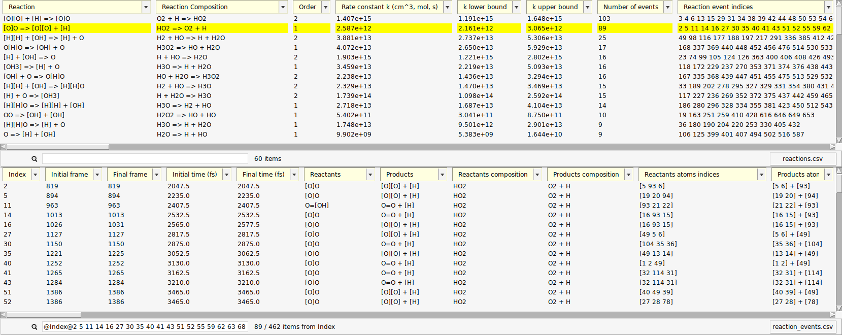
When a reaction entry is selected, the lower list automatically shows all events of that reaction. The search bar below the events list then shows the search query that is used as a filter, e.g. (“@Index@3 45@”)
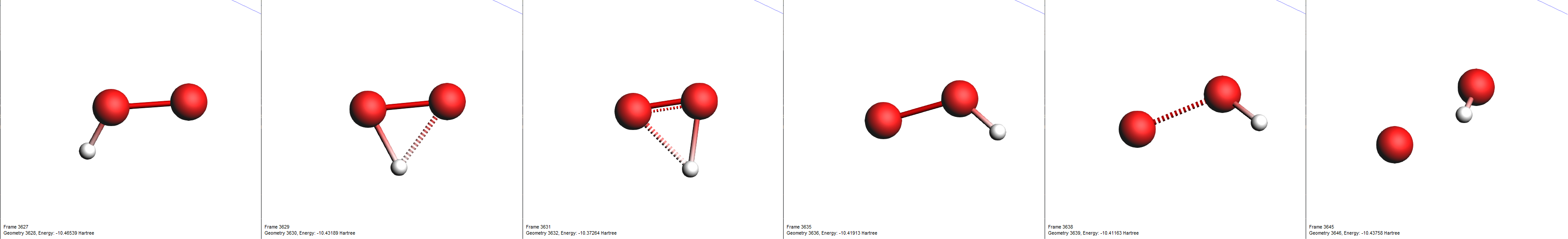
One of the reactions we expected to happen was \(\mathrm{HO_2 \rightarrow O + OH}\). Let’s use the search function to find its first occurrence.
Note
The first reaction on your list may not be identical to the reaction shown here. The first reaction will depend on the initial conditions of the simulation, which will be slightly different from those used for this particular example.
search field from the lower list@Products:[OH]Now, only reactions with a hydroxyl radical \(\mathrm{OH}\) as a product are shown. Note here, that we have used the radical’s SMILES format for filtering (“[OH]”).
By clicking an entry of the events list, AMSmovie automatically hides all atoms that are not involved in this particular event. Now, we can take a look in detail what led to the first production of \(\mathrm{OH}\).
 search field
Using the “T_stable” setting
See also
As mentioned in the introduction, the engine we used, ReaxFF, is a classical force field and therefore it does not include electrons or orbitals. Especially in our dense simulation, some unintuitive or unexpected molecules may appear, like \(\mathrm{HOHOH}\) or \(\mathrm{OH_3}\). These might be artifacts of imperfect force field parameters or actual short-lived, unstable intermediates.
In the latter case, we can make the criteria for stability more strict to filter out some of these short-lived species. This criteria is called T_stable and can be accessed in the CT2 menu as an analysis setting. T_stable is essentially the minimum amount of time a species must exist in order to be considered stable and appear in the results.
In this section of the tutorial, we will look for the unstable intermediate \(\mathrm{HOHOH}\) and increase \(\mathrm{t_{stable}}\) to see the effects on the reaction detection involving this intermediate.
@Products:O[H]O in the search field of the lower listIf we see \(\mathrm{HOHOH}\) in one of lists, it means that the intermediate was present in the simulation for longer than the time specified by T stable.
20Wait for the analysis to finish, and look look again for \(\mathrm{HOHOH}\) in the reactions list.
@Products:O[H]O in the search field of the lower listBy increasing the time threshold of stable molecules, the number of unstable intermediates detected as reaction products should have decreased.
Investigating population properties of the trajectory
CT2 enables the user to access information about the dynamics of species counts, when reactions occur over the course of the trajectory, as well as many other general quantities that describe the evolution of the trajectory over time. This information is not calculated by default but can be requested on the ChemTraYzer2 settings window. We’ll go through an example illustrating how to access these properties.
Now, our output contains a third table, as shown below.
Now, click on a few of the molecules in the third table and take a look at the generated graphs. One of the graphs you’ll notice is the ChemTraYzer2 Events Per Time graph. This is a histogram of the number of reactive events and bond change events that occur in a certain bin of frames. Adjust the display style (lower left corner) to Bar and change the bin width to 2000 to generate an image like the one below.
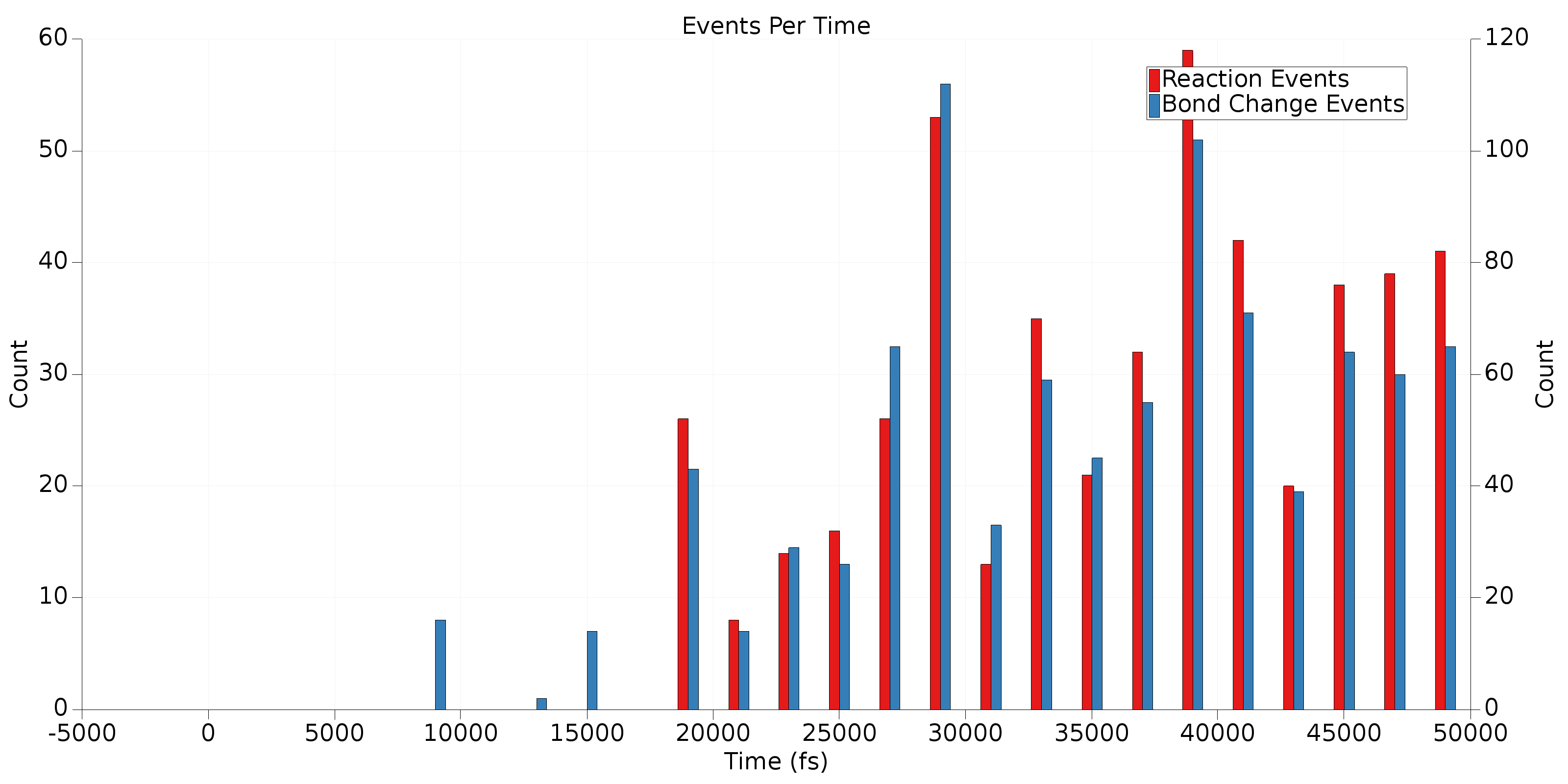
Remember, bond change events occur any time a bond breaks or forms, even if this quickly re-forms the original molecule. Reaction events are sequences of bond change events that have not been filtered out (e.g., by the T_stable criterion). This plot provides an overview of when reactions and bond changes are occurring in a trajectory. This can be useful to determine if your reactive trajectory has reached equilibrium or if it terminated before all reactions completed. In the example above, it’s clear from the high bars near the right side of the graph that this trajectory should have been run for longer. Also, in general we expect there to be more bond change events than reactive events. Some bond change events are acceptable near the end of the trajectory, but significant numbers of reactive events in this region are an indication that the final frame of the trajectory has not reached reactive equilibrium.
Finally, we’ll take a look at some common species in this MD simulation. To do that, we’ll go to the third table and sort (decreasing) by Average Count. Clicking on the top 4 molecules in the sorted table (you may have to CTRL+click to select multiple) will produce a table like the following:
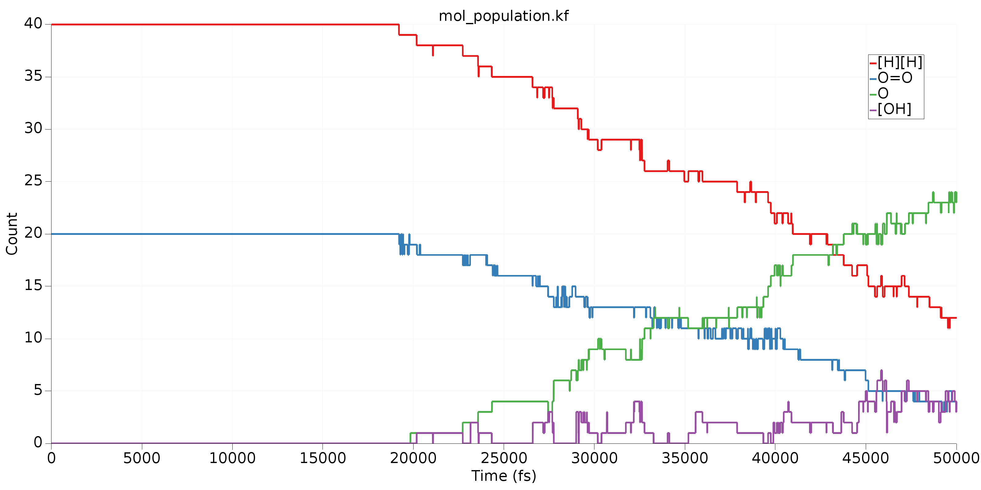
In this image, we can get a clear overview of what’s being consumed as a reactant and what’s being produced as a product. Clearly, \(\mathrm{H_2}\) and \(\mathrm{O_2}\) are reacting to form \(\mathrm{H_2O}\). The fourth species, called \(\mathrm{[OH]}\) above is an important intermediate in this reaction. Its rising population count is another indication that our trajectory is not in reactive equilibrium.
Tip
In the third table, the Mann-Kendall value attempts to capture the degree to which a species behaves like a reactant or product. All Mann-Kendall values are in the range [-1,1]. Species that behave as reactants should have more negative values, products more positive values, and intermediates somewhere around 0. The Mann-Kendall values for the 4 species shown in the graph above clearly indicate what we’d expect: \(\mathrm{H_2}\) and \(\mathrm{O_2}\) are reactants, \(\mathrm{H_2O}\) is a product and \(\mathrm{[OH]}\) is somewhere between an intermediate and a product.