Thermal conductivity from NEMD
In this tutorial the temperature-dependent thermal conductivity is calculated from a non-equilibrium molecular dynamics (NEMD ) trajectory. The AMS engine used is the UFF force field .
A heat flow is realized by running two local thermostats, heat source and heat sink, inside the same molecular structure. The heat source is set to be 10K above the target temperature, while the heat sink is kept 10K below the target temperature. From the energy collected at the heat sink over time and the cross-sectional area, the heat flux and thermal conductivity can be calculated. Both the molecular structure and the workflow were taken from the combined experimental and theoretical study E.M. Moscarello, B.L. Wooten, H. Sajid, L.D. Tichenor, J.P. Heremans, M.A. Addicoat, P.L. McGrier, ACS Appl. Nano Mater. 2022, 5, 10, 13787–13793.
The heat flux Q can be calculated as
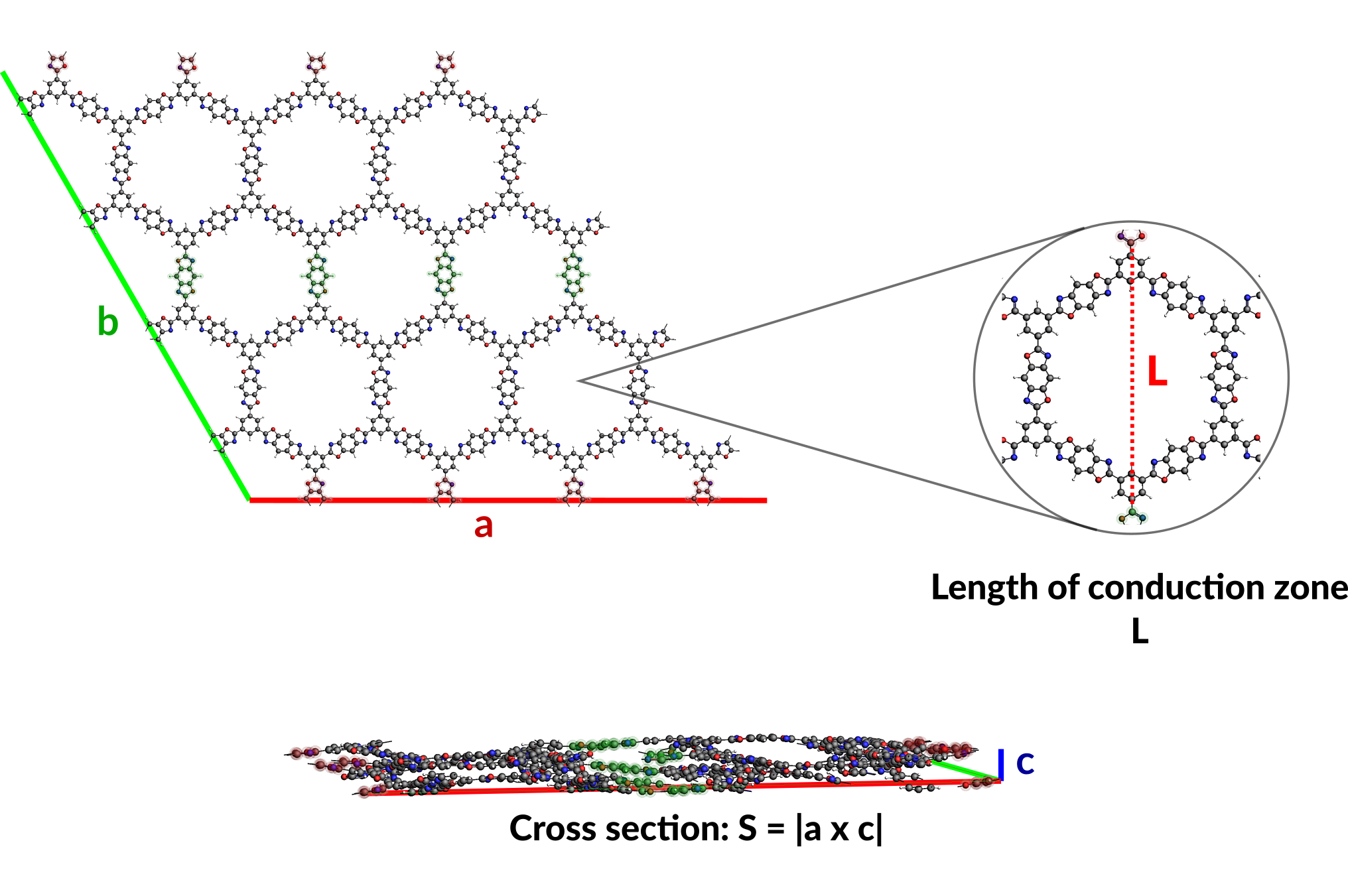
where S is the cross-sectional area. The heat flux is related to the thermal conductivity via Fourier’s law
where L is the length of the conduction zone and \(\Delta T = T_{\textrm{source}} - T_{\textrm{sink}}\).
Combining these two equations gives the thermal conductivity k as
Setup
Begin by downloading the input structure BBO_COF1.xyz. The file contains the cartesian
coordinates of a benzobisoxazole (BBO)-linked COF for which the thermal conductivity at 80K will be calculated.
Note
The periodic structure has been relaxed with GFN1-xTB (including the lattice), as described in the paper .
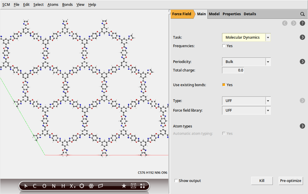
BBO_COF1.xyz and import them into AMSinput
Define a heat source and a heat sink by using regions .
 and View → Periodic → Periodic View Type → Repeat Unit Cell
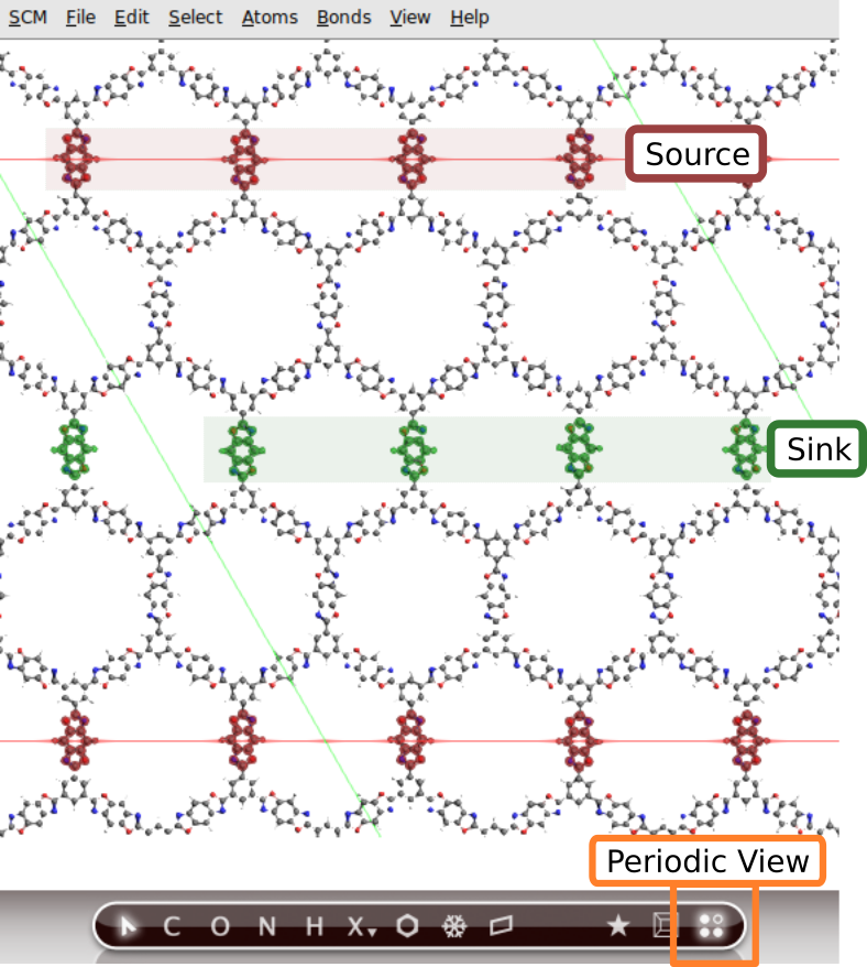
 to generate a region
source for the regionsink region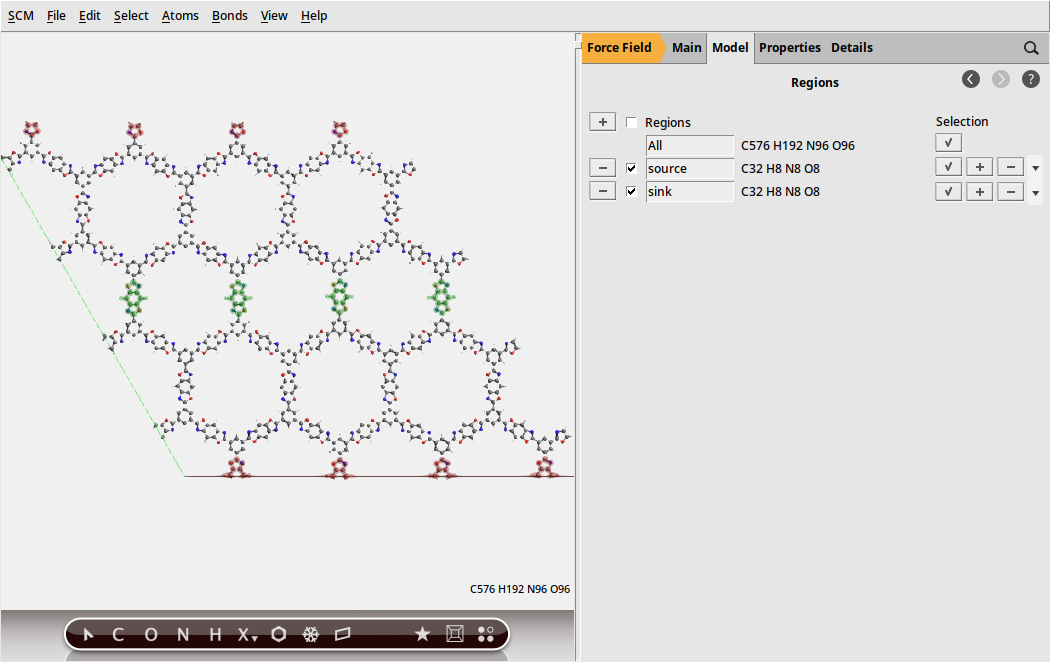
The source and sink regions can now be connected to two independent thermostats
to generate a thermostat9010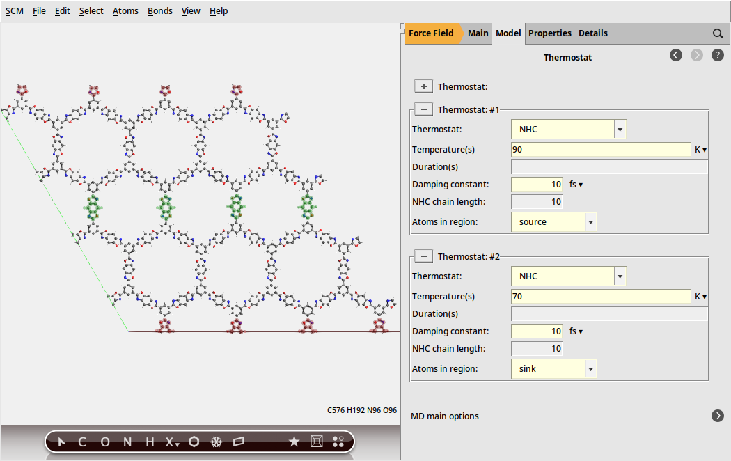
As the final step, define the settings for the molecular dynamics calculation
2000001 fs100080 K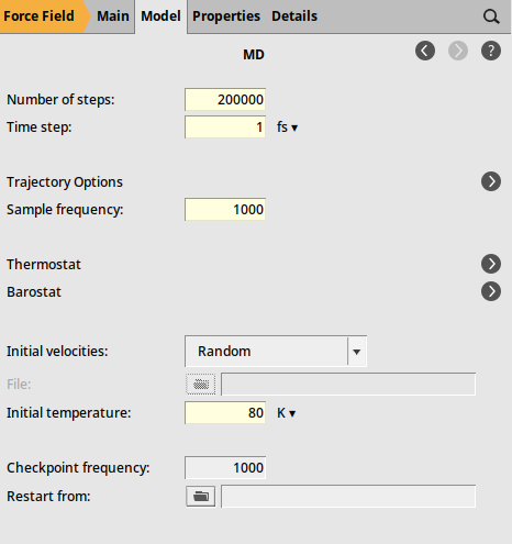
It is also a good idea to disable writing engine results files (MDStep*.rkf). For the ForceField engine, these do not contain much useful data and would needlessly take up disk space.
 next to Trajectory Options to go to the Model → MD… → Trajectory Options panel
0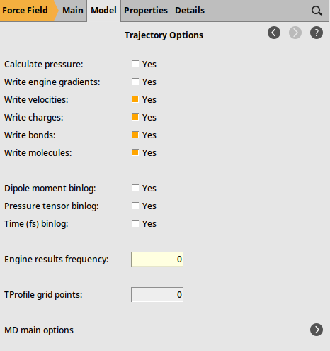
To start the calculation, do
The calculation takes around 20 minutes on a modern 12-core desktop computer.
Results
Once the calculation has finished we can view the results in AMSmovie.
 select AMSmovie
The relevant bits for the NEMD calculation are the energies of the two thermostats as well the time. To visualize these values:
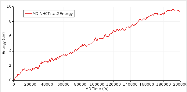
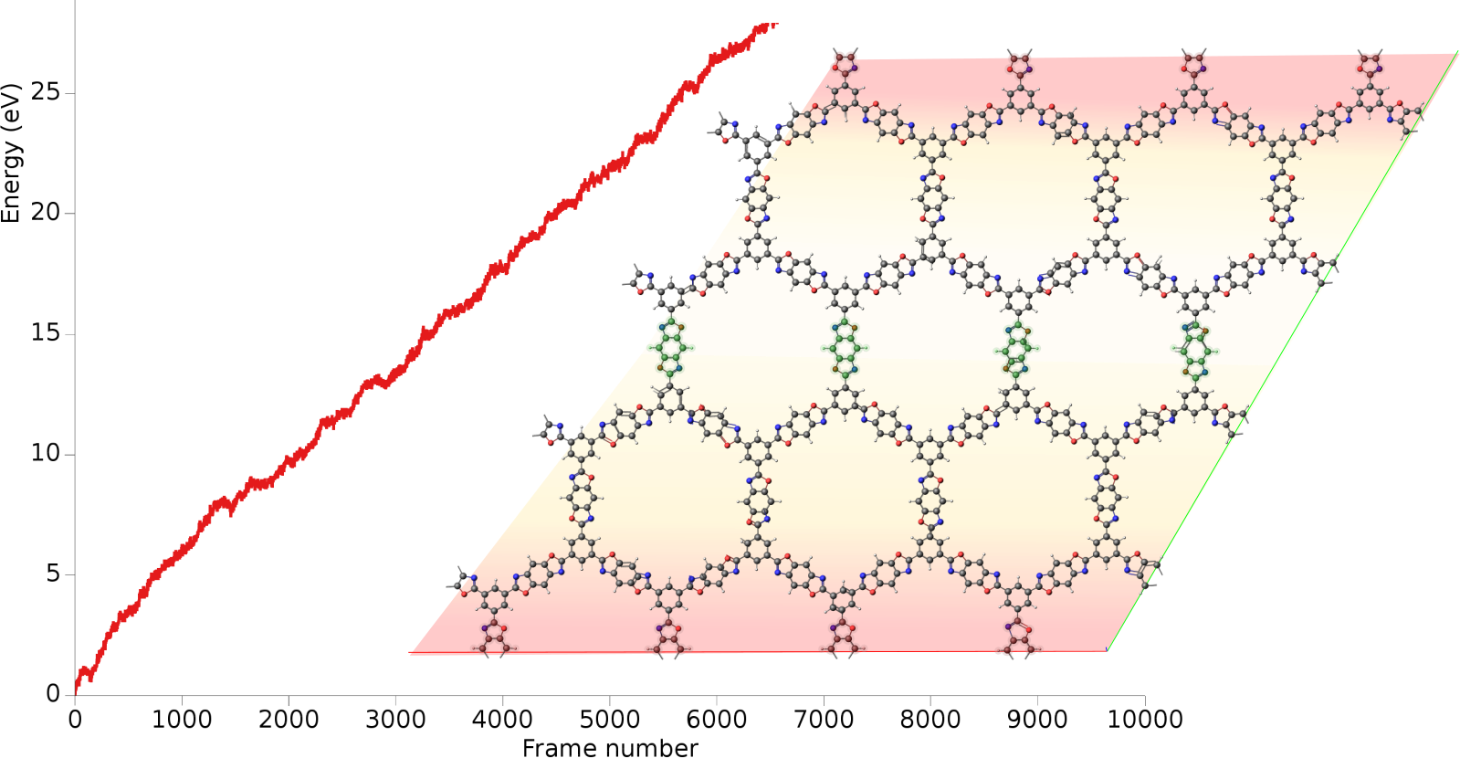
After the simulation has equilibrated, this curve should increase linearly with time. In this tutorial, we ran a relatively short simulation of 200 ps but ideally it would be run for much longer.
Starting with AMS2023, the slope of the curve can easily be calculated inside AMSmovie.
next to Name100000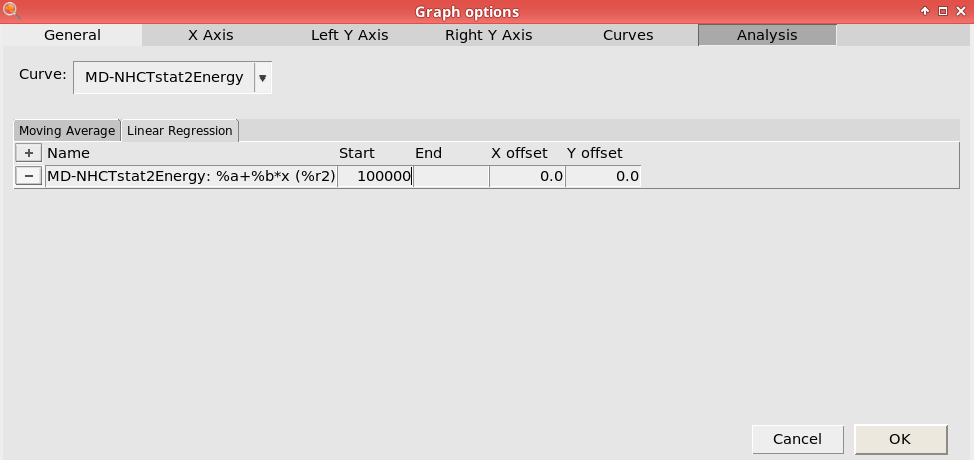
This will perform linear fit starting from 100,000 fs. Here, we consider the first 100,000 fs to be part of the equilibration period.
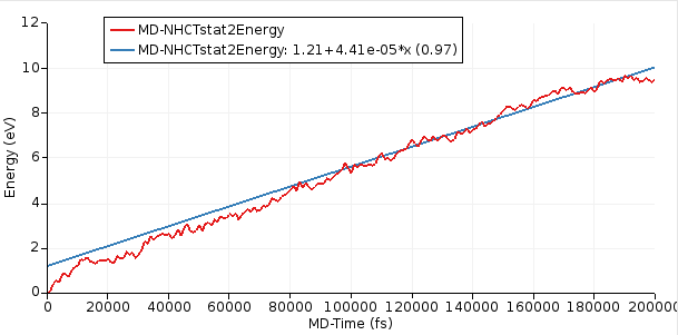
From the above figure, you see that the slope = dE/dt = 4.41 × 10⁻⁵ eV/fs = 7.07 × 10⁻⁹ J/s.
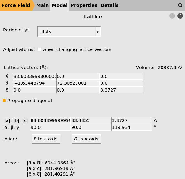
S is the cross-sectional area, i.e. the area from which heat enters the system, that can be calculated from the lattice vectors a and c of the system:
Recall the thermal conductivity k:
The factor 2 stems from the periodic boundary conditions because the heat can flow in two directions.
Inserting the above numbers (with ΔT = 90 - 70 = 20 K) yields k = 0.23 W m⁻¹ K⁻¹ (experimental value: 0.195 W m⁻¹ K⁻¹)
Note
Due to the non-deterministic nature of the MD thermostats and the fitting procedure, the result of this tutorial can vary slightly. Still, the thermal conductivity should be reasonably close to the experimental value.
Easier calculation with Python
You can also use for example the below Python script to automate the procedure of performing the linear fit and the unit conversions (you have to change the script in order to get the results for your calculation):
#!/usr/bin/env amspython
from scm.plams import *
import numpy as np


def main():
    # Unit conversion factors
    eV_to_J = Units.convert(1.0, "eV", "J")
    fs_to_s = Units.convert(1.0, "fs", "s")
    ang_to_m = Units.convert(1.0, "angstrom", "m")

    # length L and cross-sectional area S
    L = 36.15 * ang_to_m  # m
    S = 281.9 * ang_to_m**2  # m^2

    # manually calculated slope and delta_T
    dEdt = 4.41e-5 * eV_to_J / fs_to_s  # J s^-1 = W
    delta_T = 20  # K

    # automatically calculated slope
    # job = AMSJob.load_external("jobname.results")
    # dEdt = get_slope(job, min_time_fs=100000)
    # delta_T = get_delta_T(job)

    # calculate thermal conductivity k
    k = (dEdt * L) / (2 * S * delta_T)

    print(f"Thermal conductivity: {k:.3f} W m^-1 K^-1")


def get_slope(job, min_time_fs=0):
    """
    Calculates the (absolute value of the) slope of NHCTstat2Energy.

    Discards the first min_time_fs from the trajectory.

    Returns: float. The slope in W ( = J/s)
    """
    from scipy.stats import linregress

    time = job.results.get_history_property("Time", history_section="MDHistory")
    time = np.array(time)  # time in fs

    nhctstatenergy = job.results.get_history_property("NHCTstat2Energy", history_section="MDHistory")
    nhctstatenergy = np.array(nhctstatenergy)  # energy in hartree

    ind = time >= min_time_fs
    time = time[ind]
    nhctstatenergy = nhctstatenergy[ind]

    result = linregress(time, nhctstatenergy)

    # take absolute value, convert to watt (J/s)
    slope = np.abs(result.slope) * Units.convert(1.0, "hartree", "J") / Units.convert(1.0, "fs", "s")

    return slope


def get_delta_T(job):
    """
    Assume there are two Thermostats and take the difference of their temperatures

    Returns: float. The difference in temperature in Kelvin
    """
    t = job.settings.input.ams.MolecularDynamics.Thermostat
    assert isinstance(t, list) and len(t) == 2, f"get_delta_T can only be called if there are exactly two thermostats"

    delta_T = abs(float(t[0].Temperature) - float(t[1].Temperature))
    return delta_T


if __name__ == "__main__":
    main()