Viscosity: Green-Kubo relation
This tutorial will show how to calculate the viscosity of liquid benzene using the Green-Kubo relation:
where \(\eta\) is the viscosity, \(V\) is the cell volume, \(k_{\rm{B}}\) is the Boltzmann constant, \(T\) is the temperature, \(P_{\alpha\beta}\) is an off-diagonal component of the pressure tensor, and \(t\) is time. The function \(<P_{\alpha\beta}(0)P_{\alpha\beta}(t)>\) is an autocorrelation function with the average taken over all time origins and off-diagonal components (αβ is yz, xz, or xy).
The pressure tensor equals the stress tensor plus a kinetic contribution. This tutorial was also featured in our video tip of the week series
Step 1: Create a box of benzene
Create a box of 40 benzene molecules with density ρ = 0.875 g cm-3 (experimental room-temperature density of benzene) using the Builder in AMSinput.
 →
→ 
c1ccccc140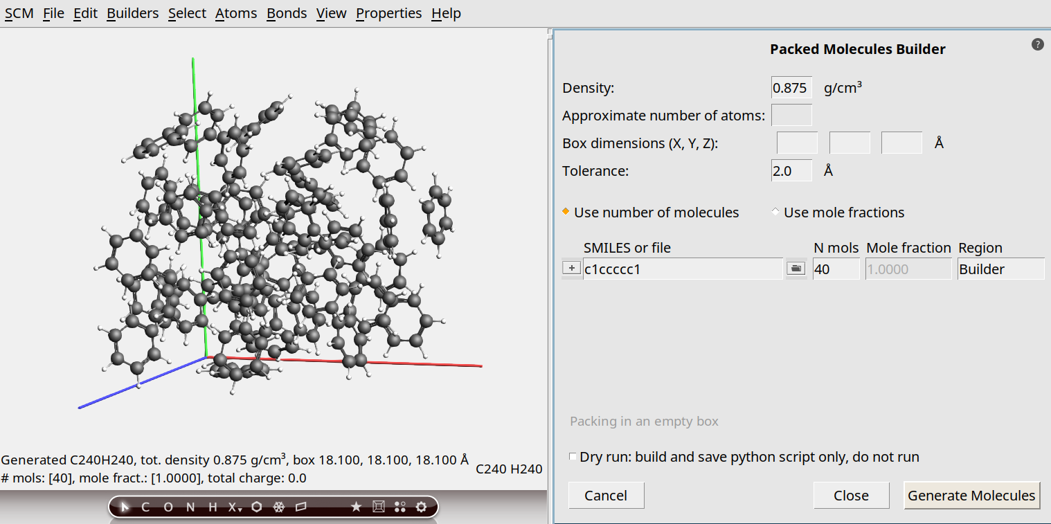
The molecules are generated at random positions and orientations. Before calculating the viscosity with a production simulation, it is very important to equilibrate the positions with an equilibration simulation.
Step 2: Set up the equilibration simulation
The next step is to set up the details of the simulation.
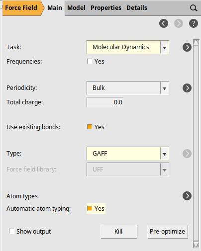
 next to Task: Molecular Dynamics
100001 fs298 K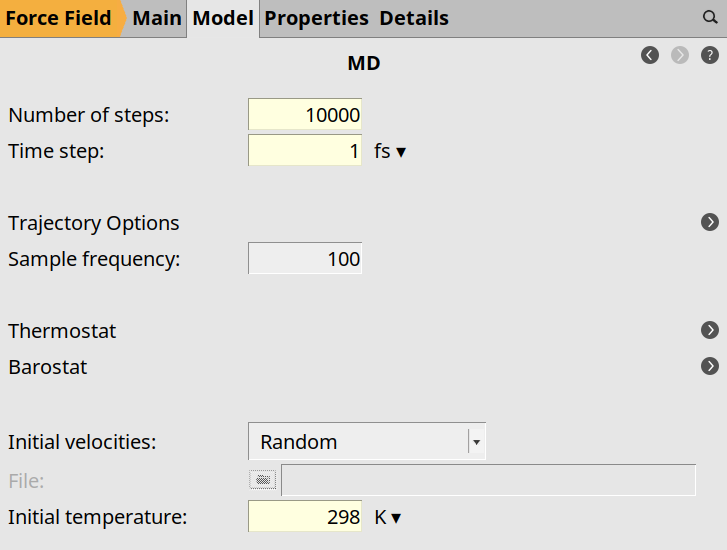 next to Thermostat
 to add a thermostat
Berendsen298100 fs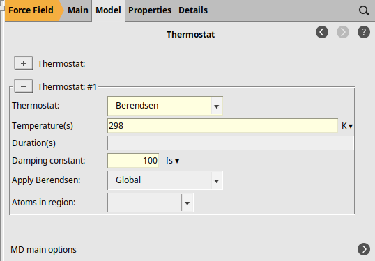
Now we will run your set-up:
BenzeneKeep the AMSinput window open while the simulation runs. It should finish in a few minutes.
When the simulation has finished, an Update Molecule button will appear at the top on your right panel. Click on it.
Step 3: Set up the production simulation
For the production simulation, we make the following changes compared to equilibration:
Increase number of MD steps
Change thermostat from Berendsen to NHC
Calculate and store the pressure tensor at every timestep (BinLog). This will be used to calculate the viscosity.
Note: The viscosity of benzene is quite low, so we can run a rather short MD simulation. Usually you would use a smaller time step than 1 fs.
400000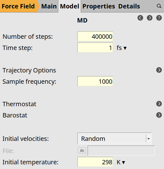 next to Trajectory Options
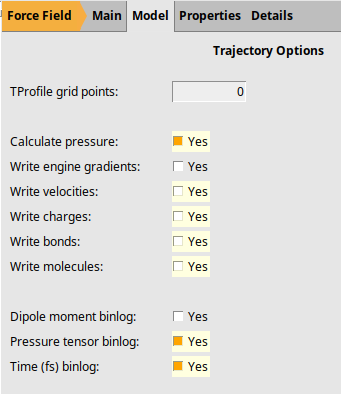
Benzene_productionImportant
Double-check that the pressure is calculated. At the start of the simulation, open the logfile (SCM → Logfile), and make sure that numerical values (and not “n/a”) is printed for the pressure. If there is no pressure, then stop the simulation and double-check that you followed all instructions.
Note
Running this calculation may take up to 2 hours.
Step 4: Analyze the simulation results
Wait until the production calculation has finished, and then open it in AMSmovie.
This brings up several graphs in AMSmovie. The bottom graph contains the viscosity as a function of upper integrand limit:
Now only the curve with the viscosity vs. time remains:
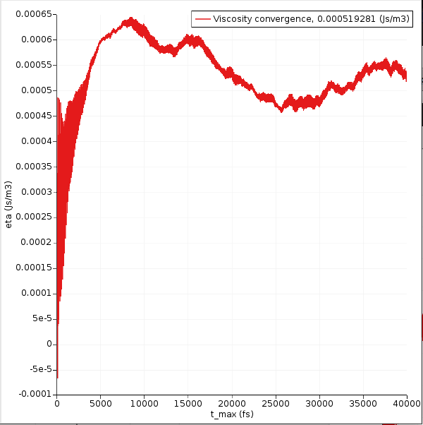
In the ideal case this graph will converge to a constant value as t → \(\infty\). This usually requires very long simulations. Your graph may look different.
Important
Even if it looks like the curve converges, the calculated viscosity may still change if you increase the simulation length.
Longer simulations are always better.
In this case, the integral seems to converge to a value of about 0.0006 J s / m 3, or 0.6 mPa s. The value that is printed in the legend is the final value, but because of noise it may be different from the average value in the “flat” region. Typically, if the curve starts to decrease in value, it is a sign of noise and not of signal.
The experimental room-temperature viscosity of benzene is about 0.5 mPa s.
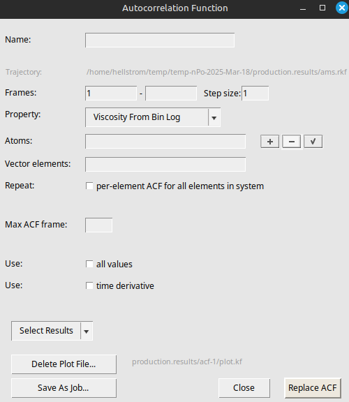
See the Python script section for how to extract the value of the viscosity with Python code. This is useful if the viscosity plot does not fully converge.
Important considerations
The simulation needs to be well equilibrated
The viscosity is often sensitive to the supercell size. Use a larger supercell with more benzene molecules for a better value.
The integral must converge in the long time-limit. You may want to increase the simulation time.
The biggest contribution to the integral comes at short correlation times. It is therefore necessary set the PressureTensor BinLog option, so that the pressure tensor is stored at every time step.
In general, make sure to equilibrate the density of the liquid first using an NPT simulation, before running an NVT simulation as above. (the above example used the experimental density, but that may not be suitable for the used force field)
Better and more reliable viscosity values can most likely be obtained using the APPLE&P or GFNFF force fields.
Python script
Check out the PLAMS example for calculating the viscosity with Green Kubo.